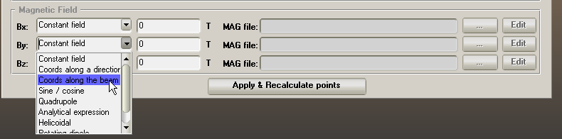
Synrad tutorial: MAG files = [Documentation for MAG files](https://molflow.web.cern.ch/node/120) # Dipole with gradient In this example we'll use a MAG file to describe a magnet whose magnetic field changes along its path. Let's make its start position at (0,0,0) and set its boundary to Z=100cm:  Instead of a constant Y field, we'll use "Coords along the beam", meaning we'll define certain points of the beam and their corresponding magnetic field. Synrad will do *linear* interpolation between them.  We have to write a MAG file.  From the documentation, the first line is: ``999999 0 0 0 10`` - 99999 is the period length (repeating the defined coordinates), we set it to a high number as there are no periods in this case - 0,0,0 is the starting point, ignored in this case (as coordinates are in S i.e. beam coordinates) - 10 is the number of data lines that follow.  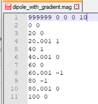The file above describes the magnetic field at S=0, S=20 etc. Note that the first and last values are held throughout the regin, so lines ```0 0``` and ```100 0``` are optional. 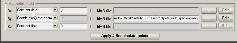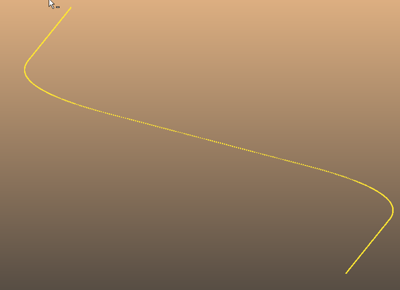Assign the just created MAG file by the Browse (``...``) button and recalculate the path:   **Important**: applying GUI values does NOT modify the .param file, you have to manually save it (easy to miss):  # Quadrupole In this example we add a straight qudrupole, also requiring a MAG file. 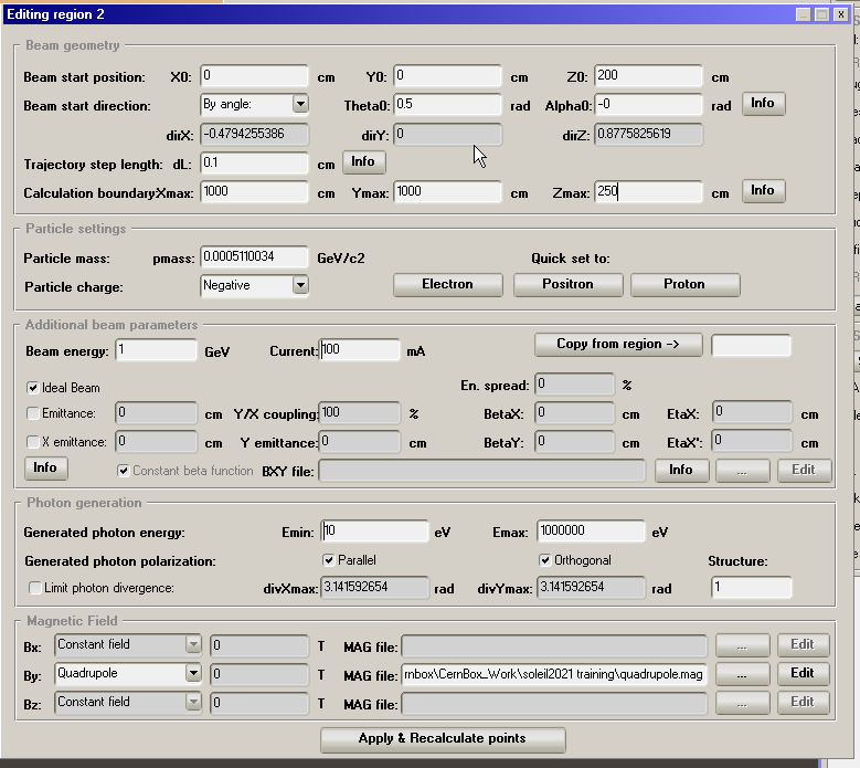- Starting point: (0,0,200) - - **The starting direction** is $theta=0.5$ (towards -X direction), description of the angles [here](https://molflow.web.cern.ch/node/118). - Boundary: Z=250cm - dL: 0.1cm Note that the quadrupole is a device that calculates the Bx, By and Bz components all at once. 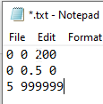So when you choose "Quadrupole" as Y component, X and Y become gray:  Let's create the MAG file: - ``0 0 200`` is the starting point (entrance) of the quad's centerline - ``0 0.5 0`` is the starting direction and orientation. $\alpha=0$ means it's in the XZ plane (no elevation angle), $\theta=0.5 rad$ rotates the quad's direction towards the $-X$ direction, $rot=0$ means it's poles are focusing. Description of the angles [here](https://molflow.web.cern.ch/node/118). - ``5 99999`` means that the quad has 5T/m gradient and is "infinitely long" (no magnetic field cutoff before the boundary). If you define a cutoff, the magnetic field will be 0 after that centerline length.   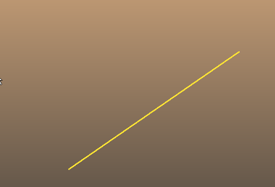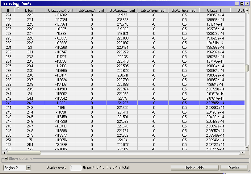After assigning the MAG file and recalculating the points, the quadrupole is rendered, so far only a straight line:  Checking its points we can see that the Orbit_B quantity (magnetic field on the ideal orbit is ~0), which is expected (quad has 0 field in its center):  ## Adding lattice functions So far our beam was ideal, i.e. 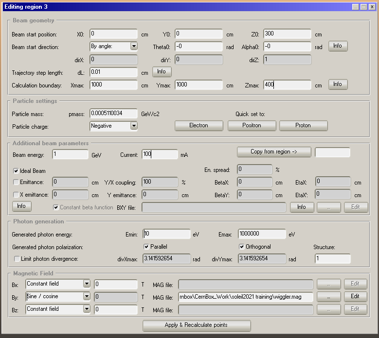zero width:  Let's add it some width with (constant) lattice functions $\beta$ and emittance:  And the photons gain some B field:  And the beam size is visible:  # Wiggler We'll place a (sinusodical) wiggler as third region. 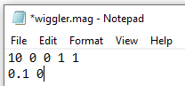- Start at (0,0,300) - Direction towards Z - dL=0.1cm - Boundary at Z=400cm - Choose sine/cosine as magnetic Y component:  MAG file contents: - `10 0 0 1 1` meaning a period length of 10cm, in the (0,0,1) i.e. Z direction, with 1 following line (1 harmonic). - `0.1 0` are the Sine/Cosine coefficients. 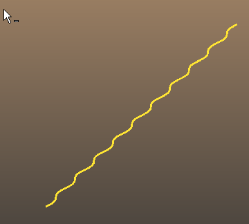This means that $B_y(Z)=0.1\sin(2\pi\frac{Z}{10cm})$  After assigning and recalculating the region, the wiggler is drawn: