Synrad tutorial: MAD sequence to Twiss file
=
# MADX
## Links
MADX website: http://madx.web.cern.ch/madx/
Latest MADX release: http://madx.web.cern.ch/madx/
MADX User Manual: http://cern.ch/madx/releases/last-rel/madxuguide.pdf
## General
Running: From command-line or Powershell, launch and type commands OR feed a `.madx` file to the binary in terminal, optionally redirect log
**MacOS** example: use ```<```
```~/madx/madx-macosx64-gnu < FCCee_t_301_nosol_53a_converter.madx > madxlog.txt```
**Windows command-line** or **Powershell** example: just separate with space
```C:\Users\marton\madx\madx-win64-gnu.exe .\Optics_FCCee_z_217_nosol_20.madx > madxlog.txt```
## Syntax
- A MADX file is a text file, just a series of case-insensitive madx commands. To write a Twiss or Survey file (the goal of this tutorial), one needs:
- a .seq file
- beam parameters
- sequence name (in the .seq file, sometimes one .seq file contains several sequences, for example LHC beam1 and beam2)
- each command must terminate with ;
- a command can span multiple lines
- separator (typically to separate argument from command) is ,
You can, if you want, skip the following part of the documentation and read only the [example](#Example)
### Variables
One can define variables:
`variable_name=100` //static value
`variable:=10*emittance` //dependent value
To execute a file from MadX (or from a MadX file): `CALL, FILE = "caseSensitive.madx";`
For system commands: `SYSTEM,"mkdir output"` or `SYSTEM, 'ls "file name.txt"'`
You can have variables but also elements, that have attributes:
`d1: drift, l=1;`
to exit: `exit;` or `stop;` or `quit;`
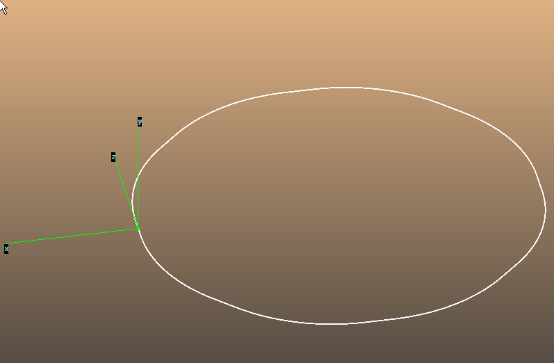
## Coordinate system
Right-hand coord. system
Local: x,y,s
GLOBAL: X,Y,Z
Global theta: right-hand around Y, so small pos. theta = small pos. X (**opposite to Synrad where ```theta>0``` means ```X<0```**)
Global phi: elevation, small pos. phi = small pos Y (**opposite to Synrad ```alpha```**)
Global psi: RH rotation around s (same as Synrad ```rot``` for quadrupoles)
Bending magnets: pos. angle: towards the right (seen from above), so towards negative X
Magnets can be rotated, for example psi=PI/2 bends down
B0 (magnetic field): positive value means magnetic field in the Y direction (bends pos. particle to the right, i.e. towards negative X)
B1 for quads (dBy/dx): pos. value horizontally focuses a pos. particle
## Built-in variables
X: position (m)
PX: horizontal canonical momentum (px/p0), refers to the reference orbit
T: longitudinal (time) offset relative to the ref. particle, pos. T means particle is earlier than ref. (T=-ct)
DELTAP: dp/p0 (diff. between reference and design momentum)
S: independent variable = beam coordinate (m)
After a TWISS command, sum variables:
LENGTH, SYNCH_1, etc
## ``USE`` command
Defines which sequence to use (by sequence name)
`sequence=seqname`
`period= position1[/position2]` //for example `range=ip1/ip2;` or `range=mb[5]/#E` //fifth mb to end
## `ASSIGN` command
`ASSIGN, echo="printhere.txt";`
then
`PRINT`
## ``BEAM`` command
Defines particle parameters, chapter 7 in manual
see below, additional options:
particle=... //defines mass and charge
otherwise mass=(in GeV, default=m_e), charge=(1->proton)
energy=(GeV)
(Gamma = energy/mass)
(Beta=v/c)
EX, EY= h/v emittance, default=1m
EXN, EYN: normalized emittance, exn=beta*ex (fix as energy ramped up?)
SIGE: realtive energy spread: sigmaE/E
KBUNCH: n. of bunches in machine, def=1
NPART: particles per bunch, default 0
RADIATE=TRUE: SR considered for bending magnets (energy loss?)
BV: beam direction +1 clockwise, -1 ccw It also flips magnetic fields (design idea: same sequence file to be used by identical charges in opposite directions -> doesn't change beam dir)
SEQUENCE: attach seq to beam by name
RESBEAM, sequence=seqname: reset all params to defaults (as non-specified might be calculated)
calculated parameters by modules:
CIRC: total circumference of machine
U0: rad. loss per turn (GeV)
To refer to params: BEAM->CIRC for example or value, BEAM%lhcb1->bv;
To get values: SHOW, BEAM;
or SHOW, BEAM%lhcb1;
## Elements
Element definition:
elementname: type {, attribute=value};
like QF: QUADRUPOLE, L=1.8, K1=0.015832;
To modify an attribute, either redefine the element or replace value: QF, K1 = 0.03;
Types:
Marker: 0-length drift like IP1: MARKER;
Drift: with length like DRIFT01: DRIFT, L=2;
Magnets: RBEND/SBEND, L=2, ANGLE=0.1, TILT=PI/2{bend downwards}, K1=...{add quad component}, E1={rot angle entrance face}, E2=, FINT={fringe field integral};
Quads: QUADRUPOLE, L=1, K1= {horizontal focusing if positive, irrespective of particle charge, K1=1/(B*rho)*(dBy/dy), TILT={PI/4 inverts H/V focussing};
HKICKER, VKICKER, L=1, KICK=d(px)/p0
RFCAVITY, L=1, VOLT={peak voltage}, LAG={0..1 repr. 0..2pi phase lag, def=0}, FREQ={in MHz}
HMONITOR/VMONITOR/MONITOR, L=1: like a drift but allows recording beam pos;
INSTRUMENT/PLACEHOLDER, L=1: representing a DRIFT but a different class
## Sequences
seqname: SEQUENCE, REFER={entry OR centre OR exit: what the AT=x refers to};
ENDSEQUENCE; pairs
entries: AT=x, FROM={AT interpreted from that element}
when USE is called, a sequence is expanded: drifts automatically created
## SURVEY module
Element coordinates in global reference system
SURVEY, SEQUENCE=seqname, FILE=outputname.txt;
additional params: X0, Y0, Z0, THETA0, PHI0, PSI0 -> only reference changed, no effect on beam
if no output file, results written in internal table named SURVEY
## TWISS module
To calculate lattice functions
Parameters:
`SEQUENCE=seqname` //Sequence to use
`RANGE=start/end` (default #S/#E) //optional
DELTAP=0.001 (rel.energy error) or range: DELTAP=0.001:0.005:0.01
CENTRE: calc functions at center of elements instead of end
FILE: output filename
KEEPORBIT: remember beam at start and at all monitors
when successful, SUMM summary parameters (tunes, chromaticities, etc) vs selected deltaP
also creates TWISS table to store results
You can also define initial values:
BETX= BETY= required.
ALFX= ...
DX= DPX= DY= ...
PHIX= PHIY=
## Example
In many cases, to convert a `.seq` to a Survey and Twiss file, you just have to modify the script below.
Assuming `fcc.seq` is the input sequence, containing the sequence called "FCC"
```
call,file="fcc.seq"; !load sequence first
Beam, particle=electron, sequence=FCC, energy = 182.5, ex=1.46e-9, ey=2.9e-12, sige=0.0015, bcurrent=0.0054;
use,sequence=FCC;
select,flag=twiss,pattern=".",column=NAME,KEYWORD,PARENT,S,L,X,Y,Z,PX,PY,ANGLE,K1L,TILT,betx,bety,dx,dpx,alfx,alfy;
survey,file=fcc_survey.txt;
twiss,file=fcc_twiss.txt;
stop;
```
particle energy in GeV, current in A
# Step by step `.seq` -> Synrad+ example with LHC
LHC main parameters: https://cds.cern.ch/record/304825/files/p61.pdf (for the script)
LHC optics: https://molflow.web.cern.ch/sites/molflow.web.cern.ch/files/soleil2021/soleil2021_source_files/synrad/STANDARD_LHC_LS2_01-APR-2021_encrypted.zip (password-protected ZIP as input, use [7-Zip](https://www.7-zip.org/) to extract)
First we create a .MADX file, which is just a list of commands to be fed to MADX on the command-line:
```
call,file="STANDARD_LHC_LS2_01-APR-2021.seq"; !load sequence first
Beam, particle=proton, sequence=LHCB1, energy = 7000, ex=2.5e-10, ey=2.5e-10, sige=4.5E-4, bcurrent=0.53;
use,sequence=LHCB1;
select,flag=twiss,pattern=".",column=NAME,KEYWORD,PARENT,S,L,X,Y,Z,PX,PY,ANGLE,K1L,TILT,betx,bety,dx,dpx,alfx,alfy;
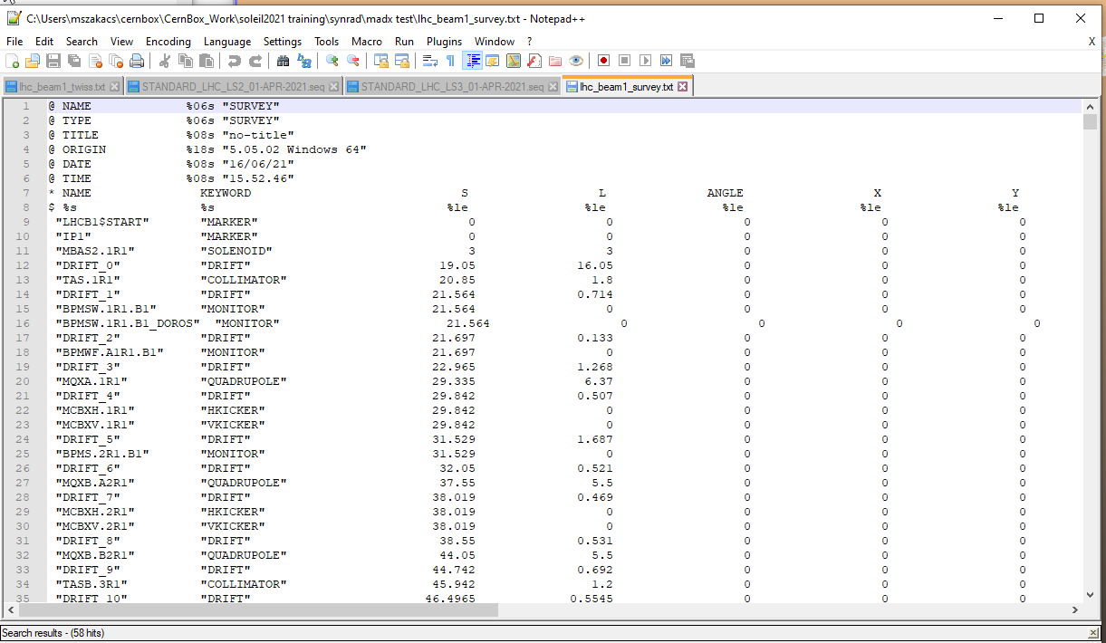
survey,file=lhc_beam1_survey.txt;
twiss,file=lhc_beam1_twiss.txt;
stop;
```
To run it, we need a Powershell in the directory with the `.seq` file.
In Windows10, SHIFT+Right click in the current directory **on an empty area of Explorer** (not on a file):
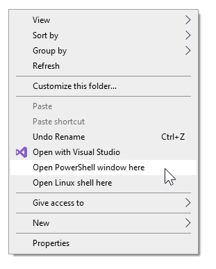
The following command calls MadX, feeds the `.madx` file above, and prints output to a `.txt` file:
```
C:\Users\testUser\madx\madx-win64-gnu.exe .\lhc_converter.madx > lhc_convert_log.txt
```
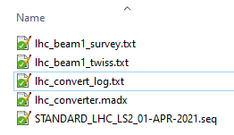
You should see the output, the Twiss and the Survey files as output:
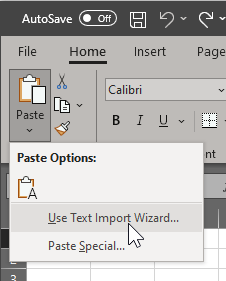
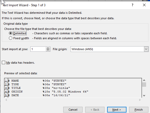
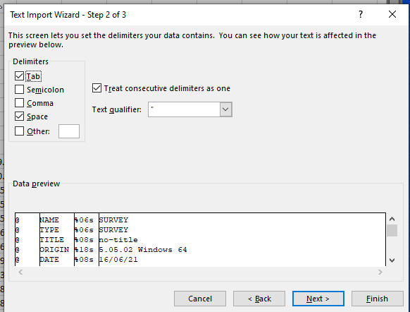
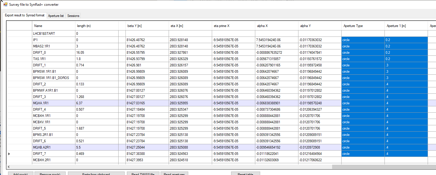
You can import the Twiss file to Opticsbuilder (Read Twiss button.)
The sequence of elements and the beam paramaters will be read and filled out:
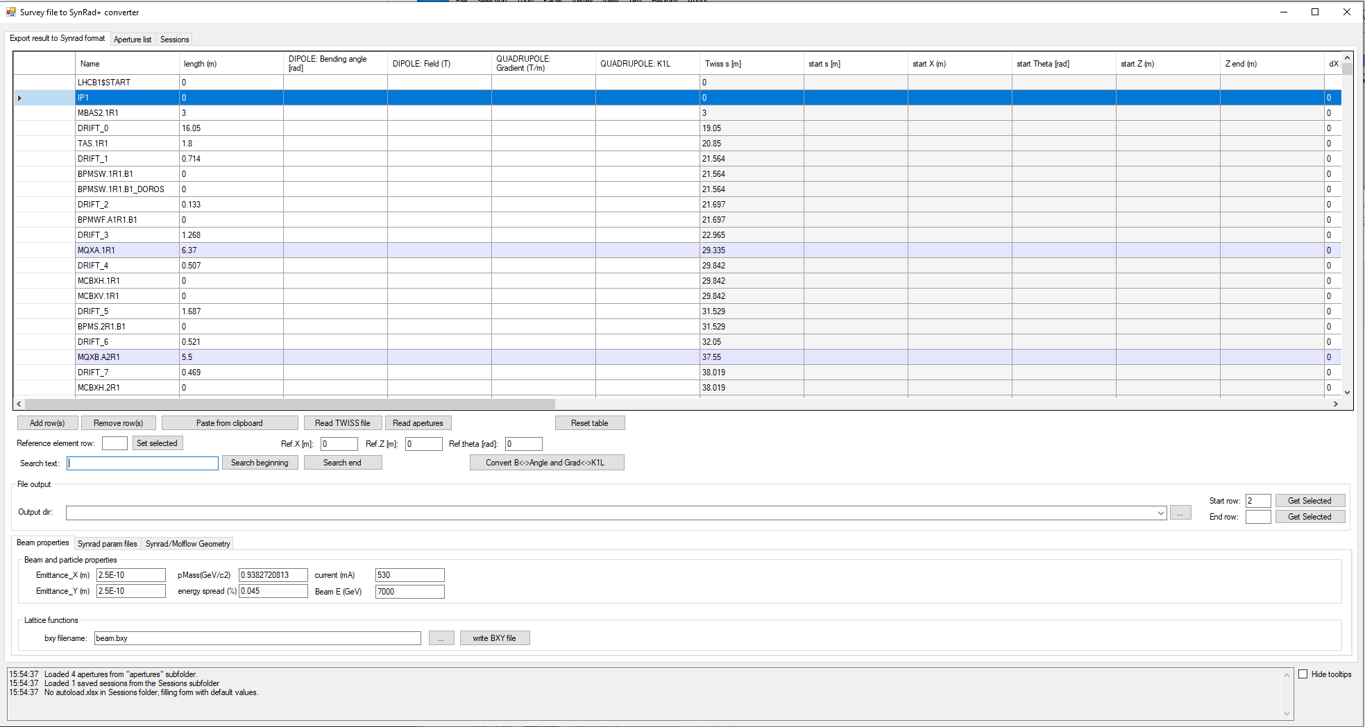
Set IP1 as reference row, which will calculate the positions of the remaining elements:

Set IP1 as start row (the previous row contains the lattice functions at the start, so it can't be the export start), then select IP2 as export end. You can search for the term IP2:

It should look similar to this with start and end set up: (if not defined, first/last lines will act as start and end)
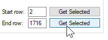
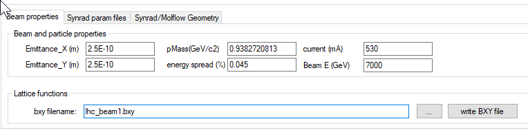
Choose an output directory for opticsbuilder. Green background means the directory exists, red that it will be created:

Click "write BXY file", then switch to the "Synrad param files" tab and click write param files:

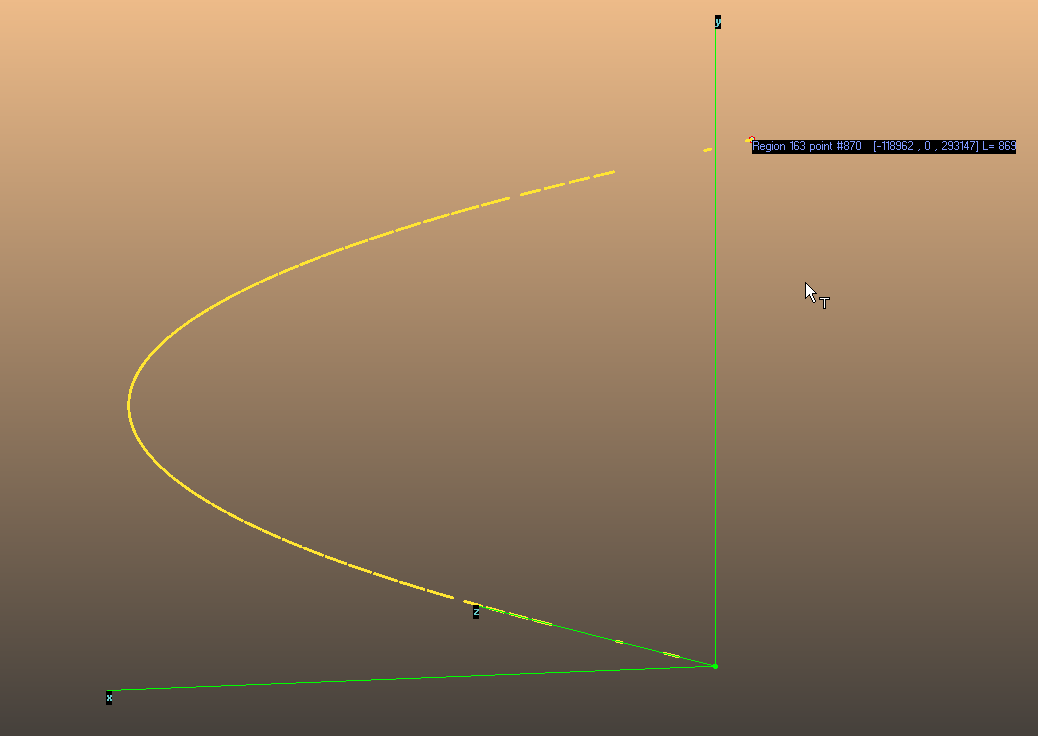
Using Regions/Load, load all files to Synrad (multi-select is allowed in the file open dialog):
## Adding aperture
The last step is to add a geometry (walls) to the imported optics.
### Manually
In this case you will use the table editor built-in.
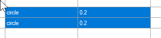
Just add an aperture type to IP1, in this simple example circle with 0.2m radius:
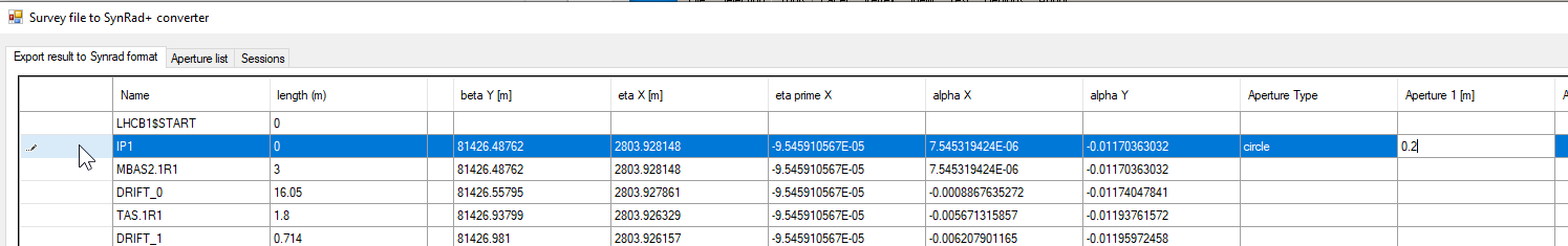
You don't need to fill all elements with an aperture, as if the field is empty, the lastt aperture type will be continued.
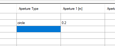
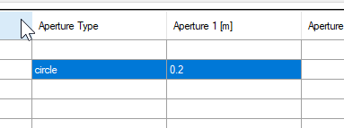
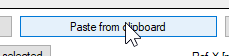
Nevertheless, you can copy the two cells and paste it, then copy the 2x2 pasted cells and paste it, and so on. CTRL+C works for copying, CTRL+V works for cell text but not for multiple cells, use the "paste from clipboard" button with the paste target's top left cell selected:
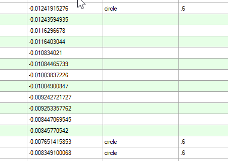
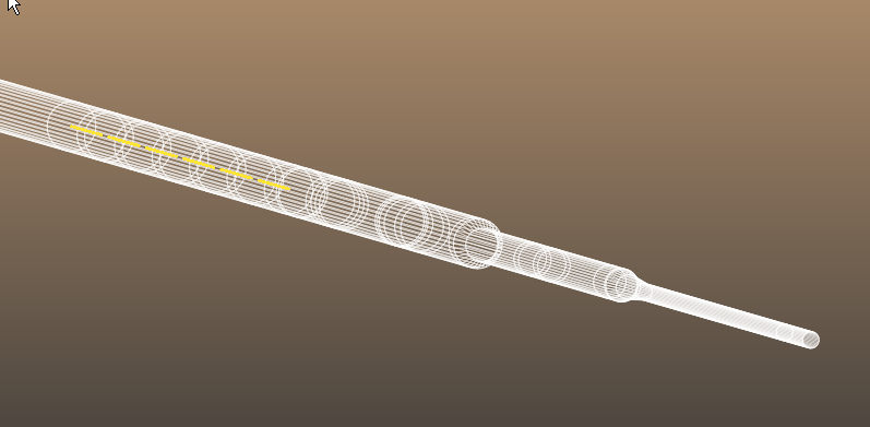
The example above has aperture defined for evfery line, below is a circle with .6m radius, continued through several dipole and drift elements:
Fill in the remaining geometry parameters, or leave them on default and click "Write geometry file":
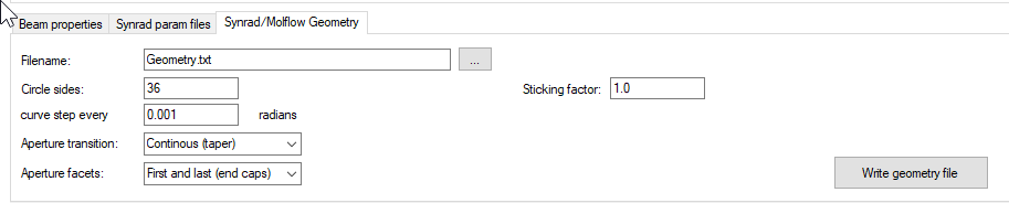
A message confirms if geometry was saved.

In Synrad+, with the optics already loaded, click File/Insert geometry/To current structure:
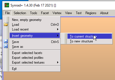
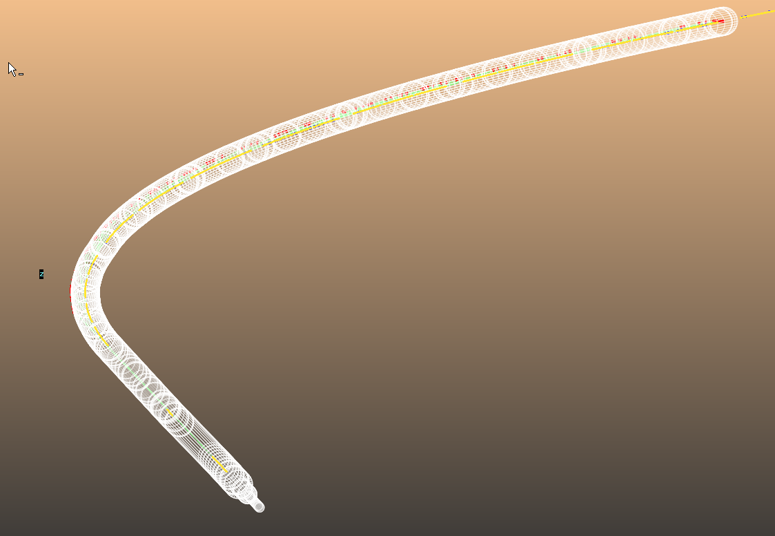
And Synrad should load the aligned geometry.
### By file
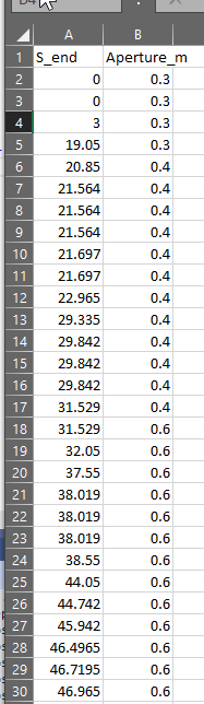
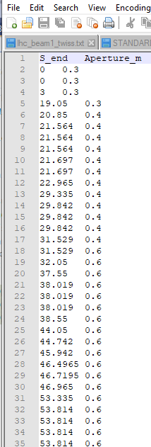
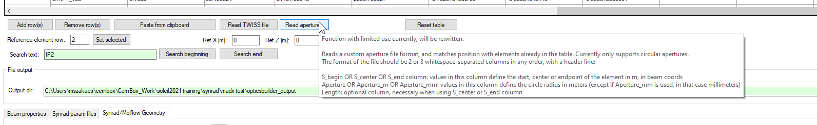
There is a method to use an external file that assigns circular apertures with user-defined radius to S poistions that match the already imported Twiss file.