310 views
Opticsbuilder: build Synrad optics from sequence === [Opticsbuilder downloads](https://molflow.web.cern.ch/content/opticsbuilder-downloads)
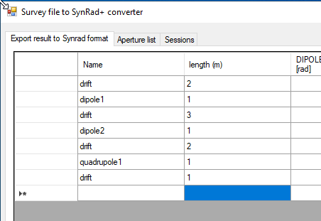
 # Adding elements First fill names and lengths: ![](https://codimd.web.cern.ch/uploads/upload_66aafa8349eb9aad21c44af72678f659.png) 
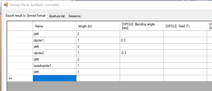
Add physical parameters: ![](https://codimd.web.cern.ch/uploads/upload_84626ff29f03c1dab39ea6321f1c56d7.png) 
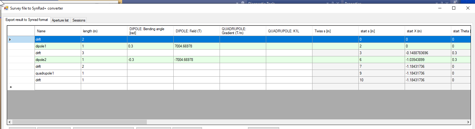
Set reference point by selecting a line (the first in this example), this is important as it will calculate element positions: ![](https://codimd.web.cern.ch/uploads/upload_1e8be05914f9217082cb39629ae9fd24.png) ![](https://codimd.web.cern.ch/uploads/upload_a3a08a1cc6e846923cb7e5d245f684db.png) The grey fields show the calculated element positions: ![](https://codimd.web.cern.ch/uploads/upload_1e9ad102a90a6270412ef168e891a2e6.png) # Adding lattice functions They are required for a Synrad simulation (ideal beam not supported) ![](https://codimd.web.cern.ch/uploads/upload_805e3c68e2e666023f40870e1db2ebdb.png) 
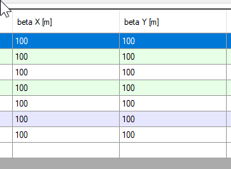
They are in meters, they must be positive.
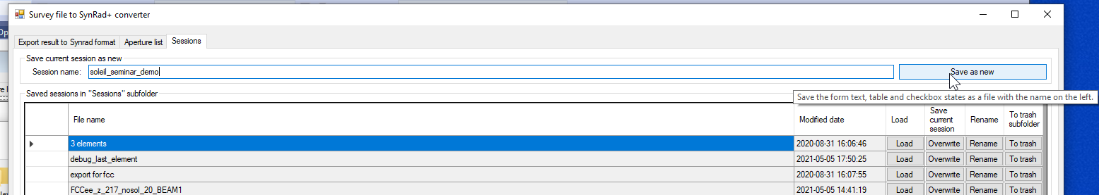
 # Saving session Opticsbuilder has a session manager, allowing you to save/load your work. ![](https://codimd.web.cern.ch/uploads/upload_216b7f8e2bd1e352210c6ac66803df55.png) # 
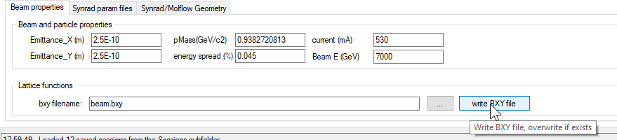
Writing lattice functions file (.bxy) First you have to write a BXY file, to be loaded by Synrad's `.param` files. ![](https://codimd.web.cern.ch/uploads/upload_82dc7f675a33784f81385b6b92cf3bdc.png) # 
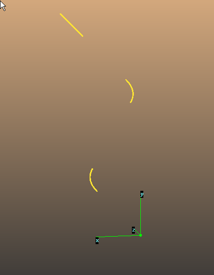
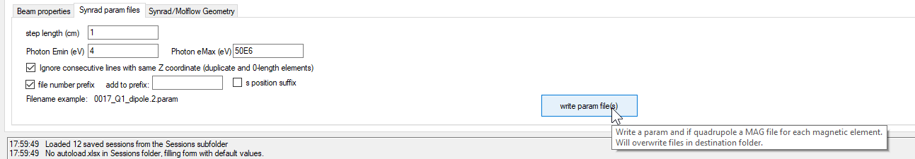
Writing Synrad regions (.param and .mag)
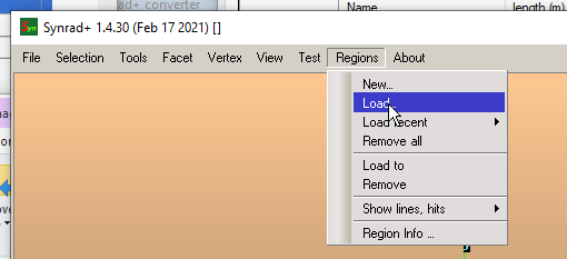
 ![](https://codimd.web.cern.ch/uploads/upload_28fcf68695a19e61a668892e1ec8b234.png) # Opening in Synrad Use the Regions/Load command... ![](https://codimd.web.cern.ch/uploads/upload_0281ea3f03b05a076bd2b15888bc2593.png) you can select all files at once: ![](https://codimd.web.cern.ch/uploads/upload_ec77aa9704226d6245d9ad6069e2da3d.png) 
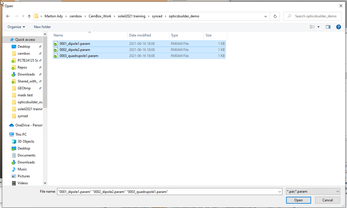
Synrad will load the magnetic regions. ![](https://codimd.web.cern.ch/uploads/upload_8852029b2df041f2b842dacdb4068444.png)