Synrad tutorial: photon simulated desorption
=
[Link to documentation](https://molflow.web.cern.ch/node/139)
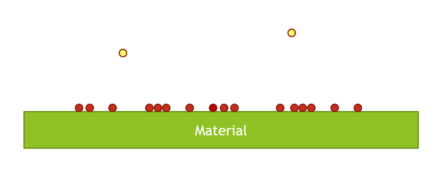
# Intro to PSD
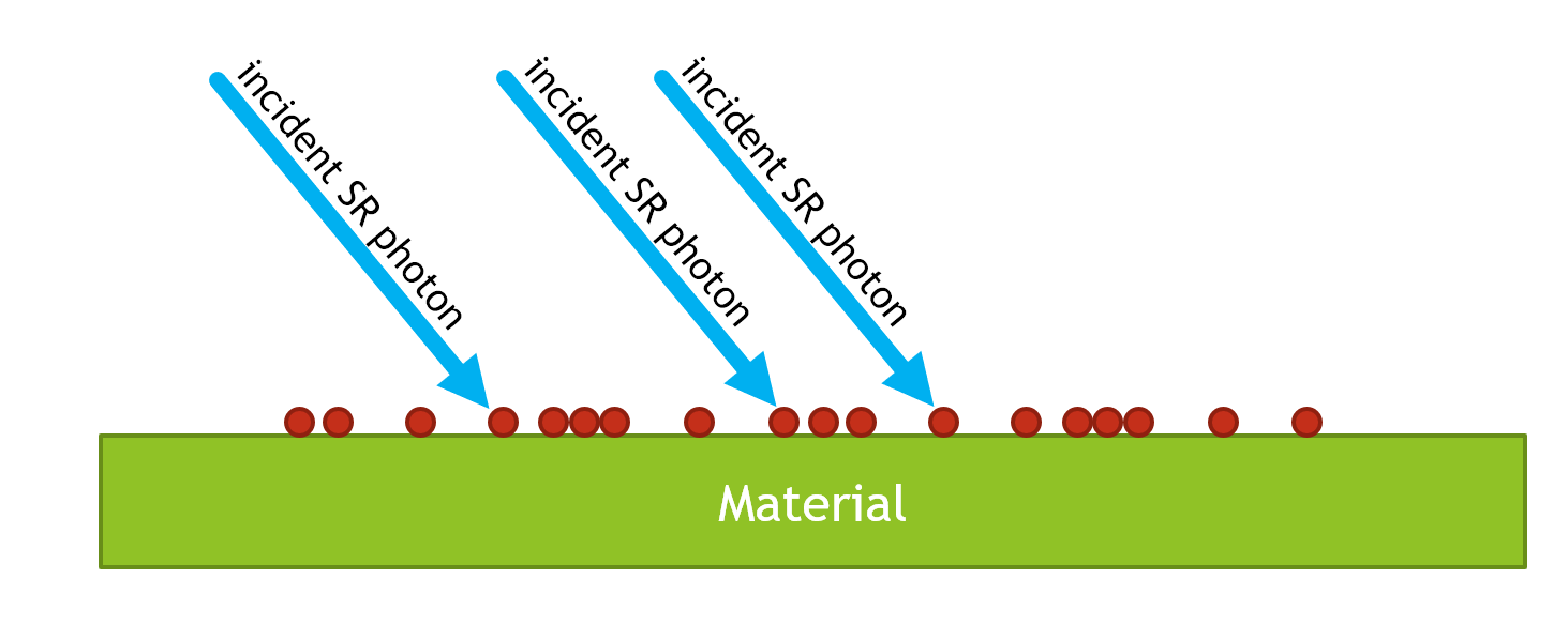
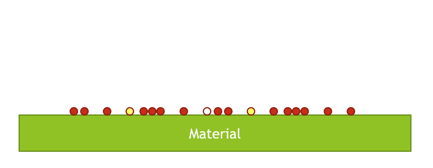
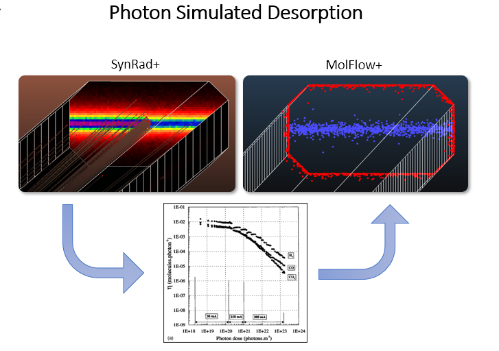
Physical process illustration:
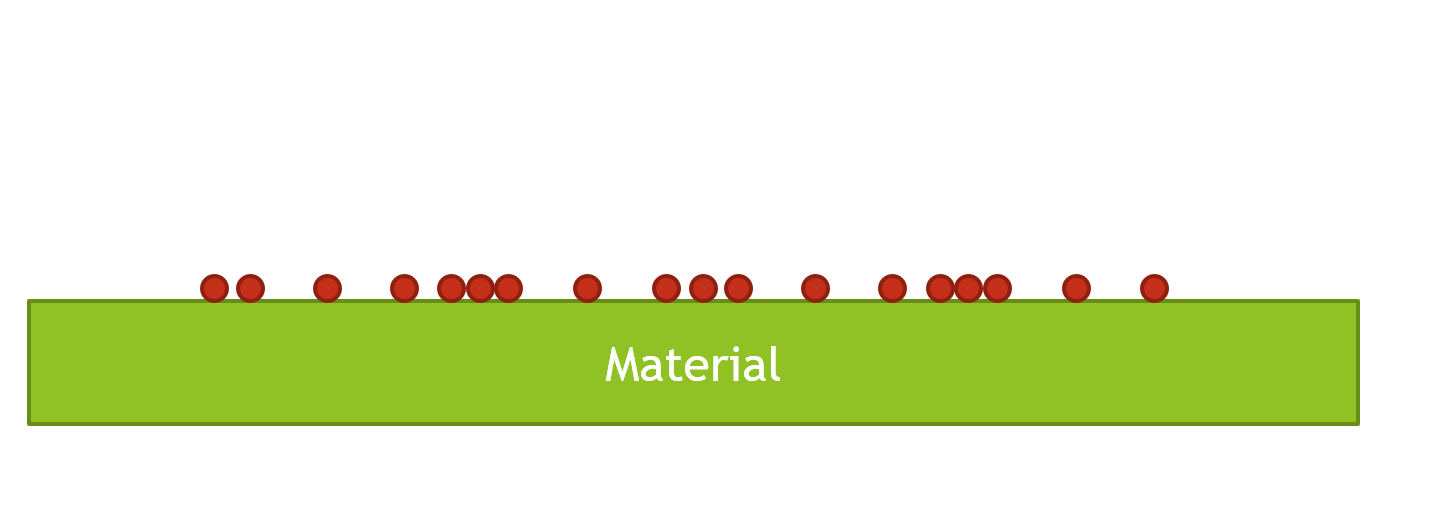
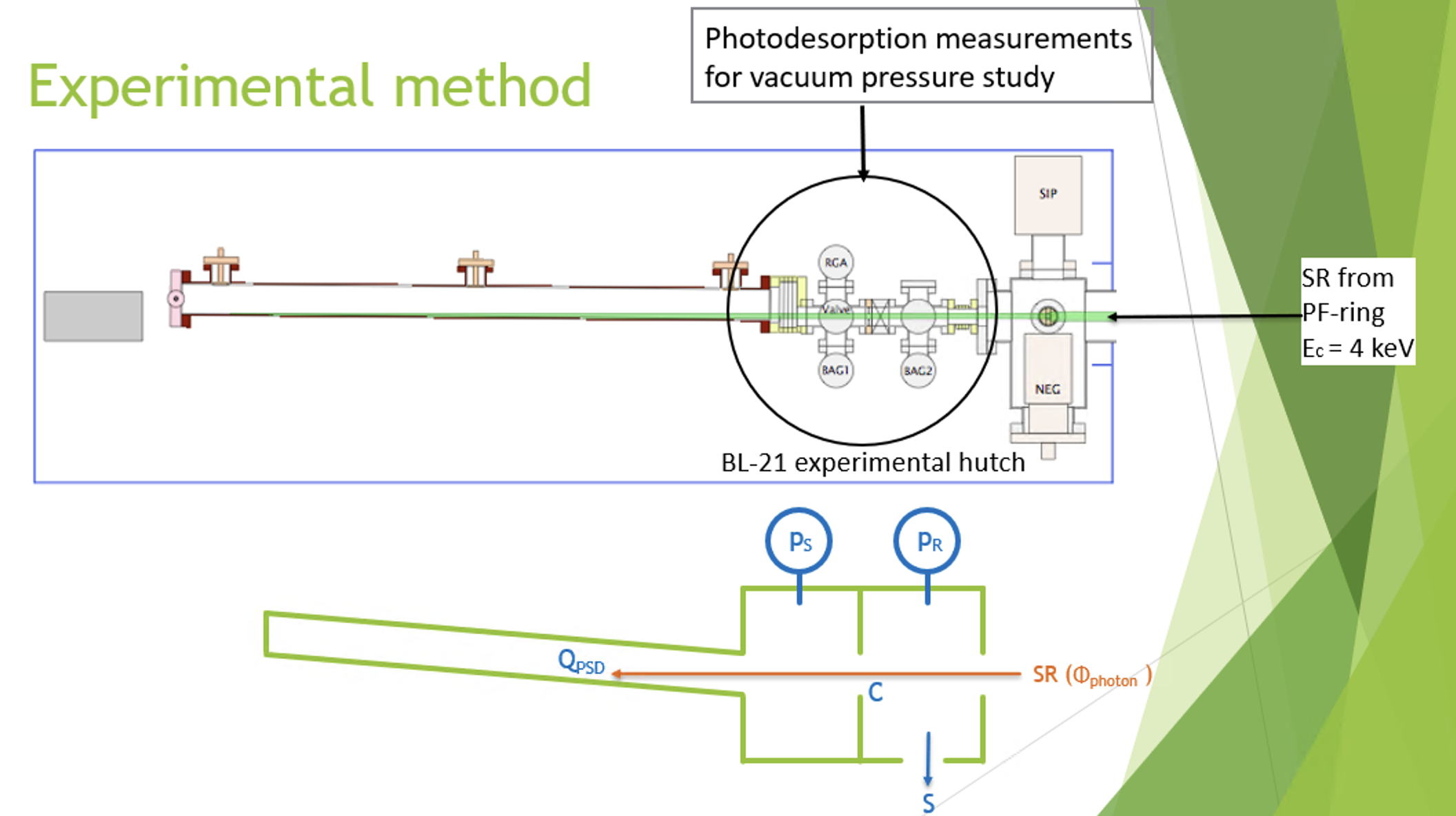
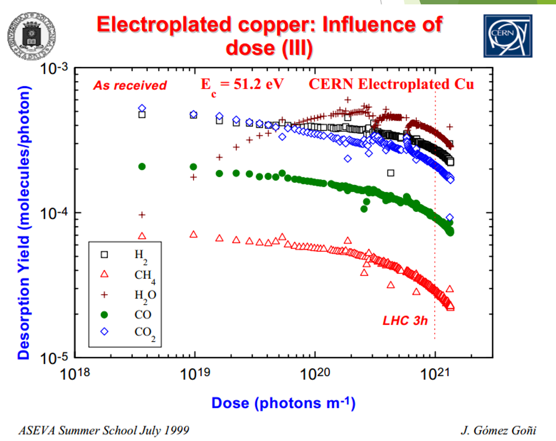
Measurement:
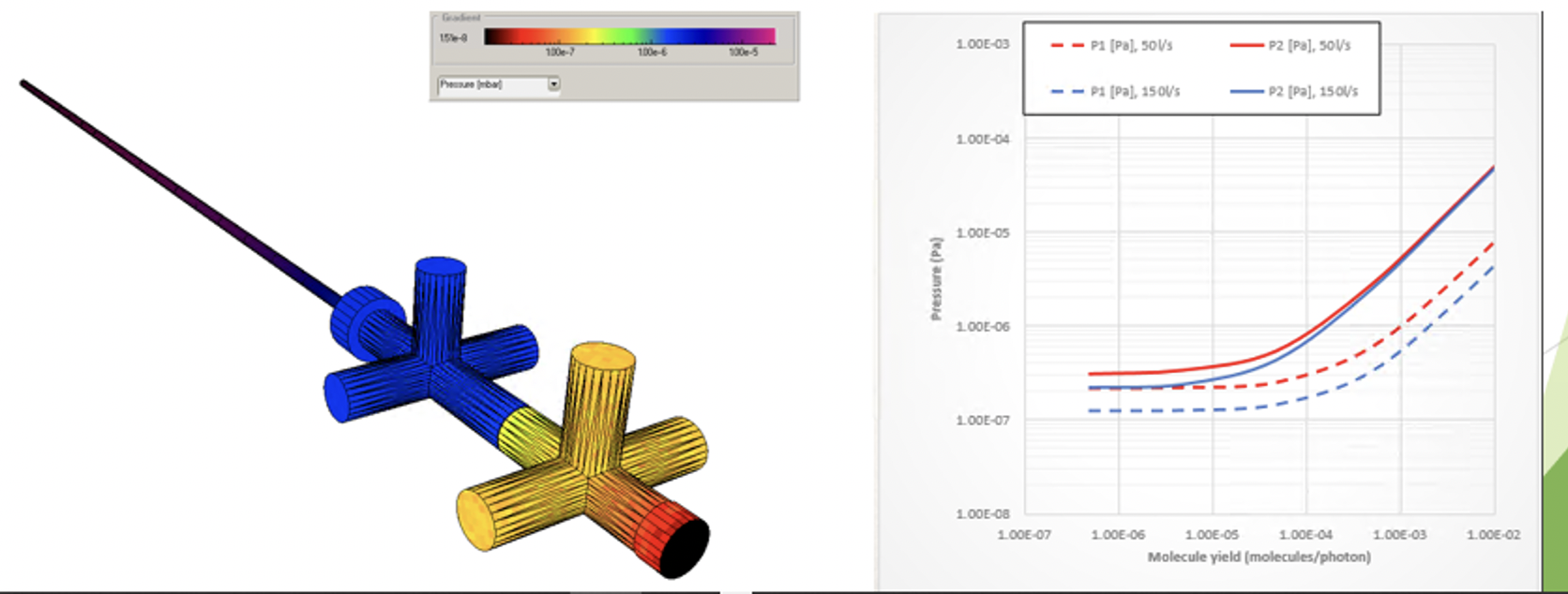
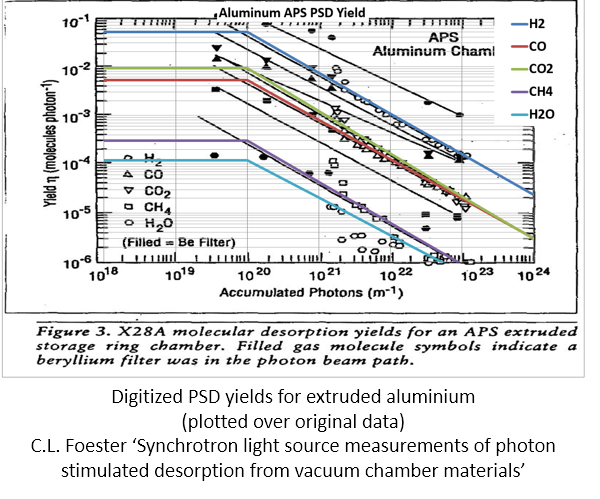
PSD data:
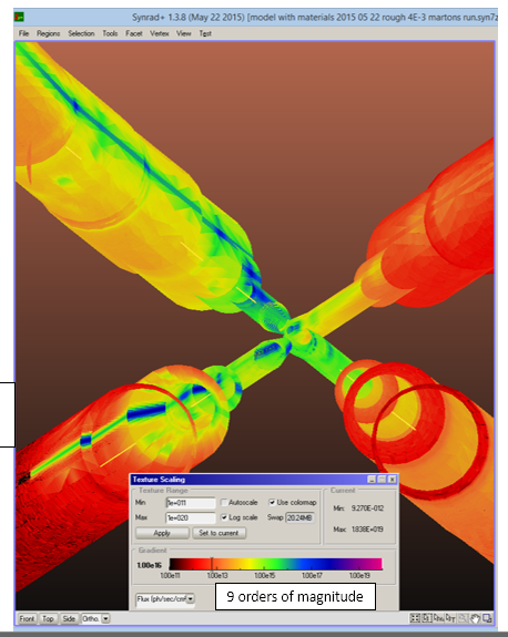
# PSD in Synrad/Molflow
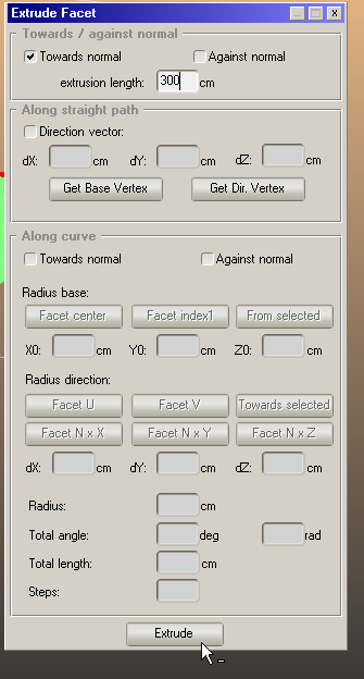
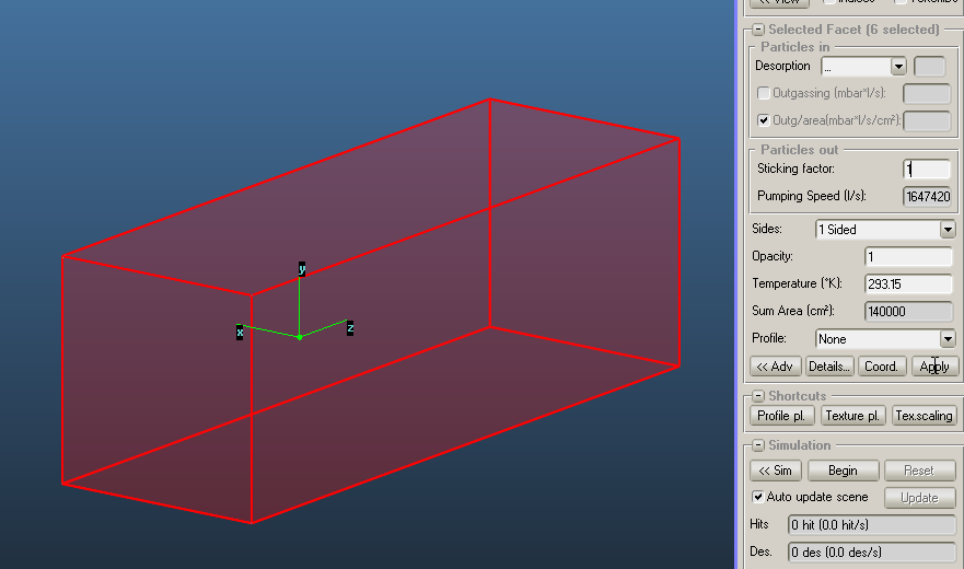
# Extruding the target to create a box
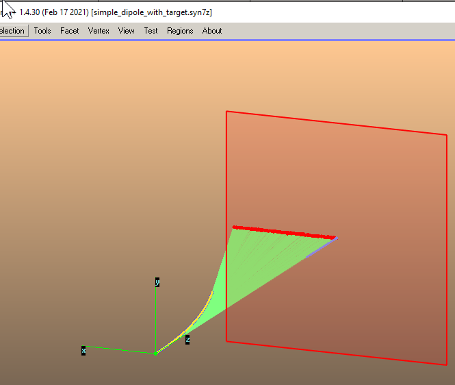
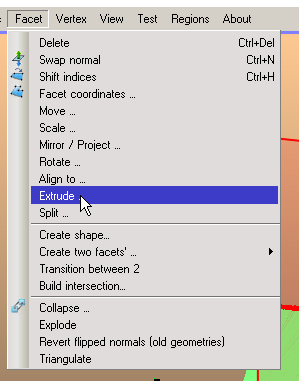
The target is already pointing towards the source, so we extrude it by 300cm (it's at Z=200cm)
And we ge ta closed box:
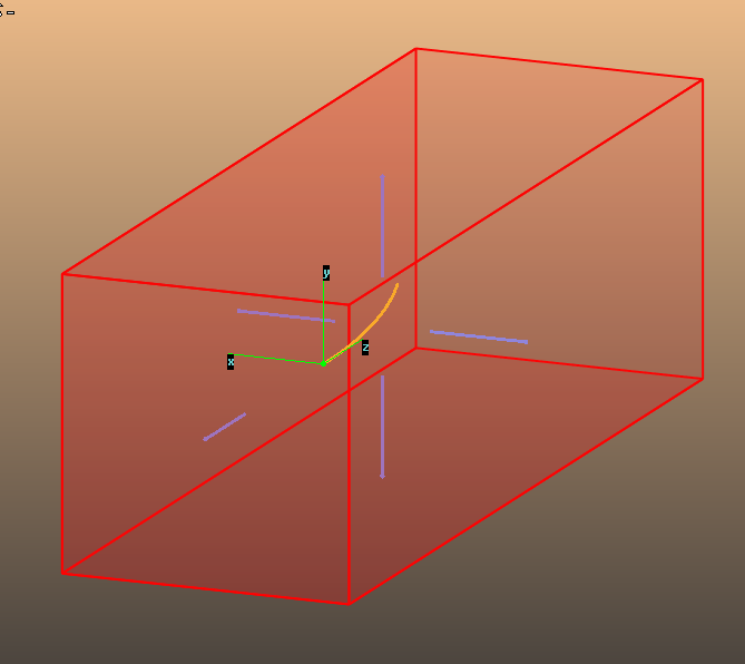
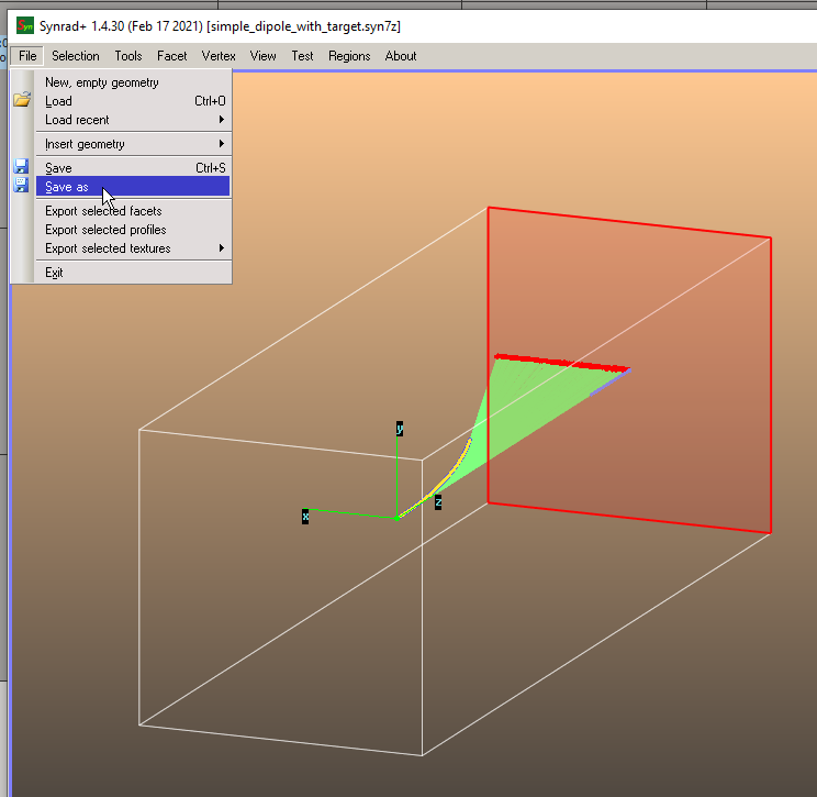
Let's run the simulation and save the file.
# Inserting in Molflow
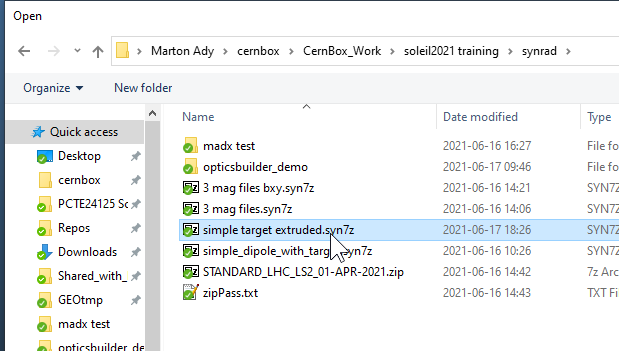
We simply open the original Synrad file:
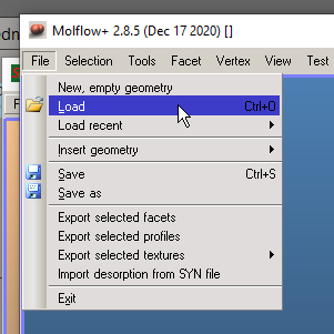
Molflow can open Synrad geometries:
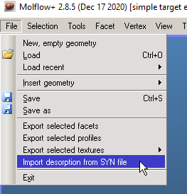
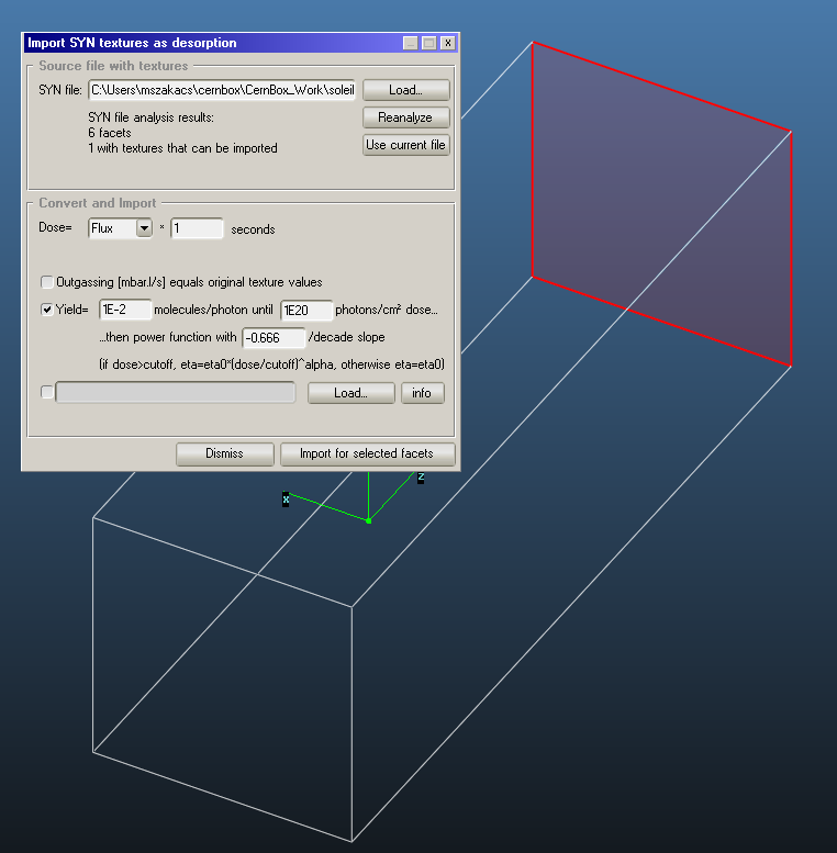
Then we "import" desorption (start the PSD conversion process):
Since we opened the Synrad file, we'll choose "Use current file":
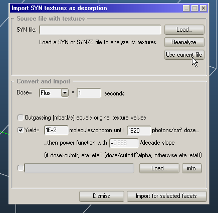
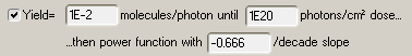
And we'll imitate a simple curve by a simple equation:

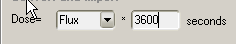
Time is 1h (3600 seconds), the longer the system conditions, the better:
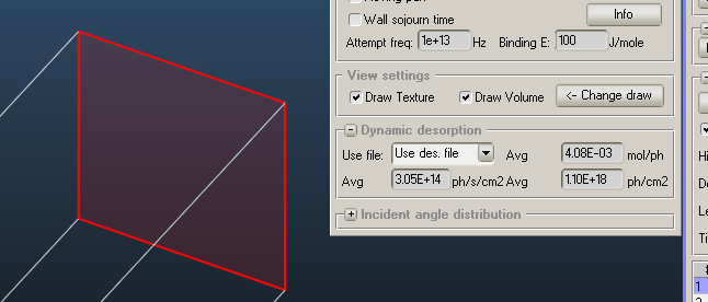
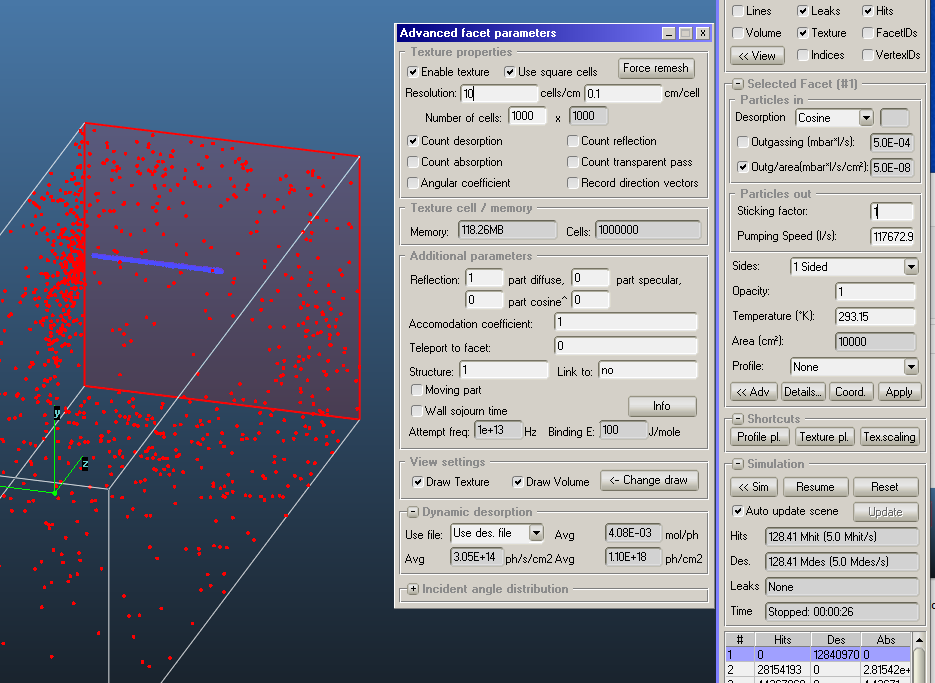
The facet advanced parameters show that it worked and give some diagnostic info:
# Run a simulation
We currently want to diagnose PSD, so we'll set sticking=1 on all facets:
The simulation looks more or less fine, particles come from where they should:
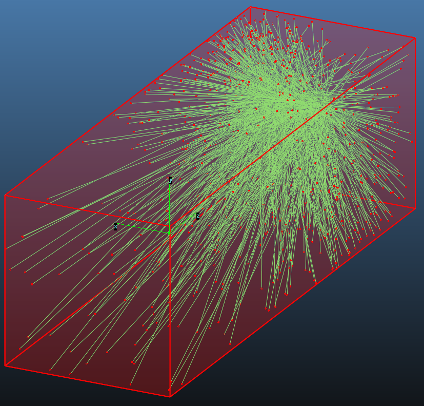
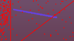
Turning on Hits view and zooming on the source, we can see that molecules are created at irradiation locations:
Let's, however, create a desorption counting texture to visualize desorption:
# Result
On linear texture scaling (Synrad vs Molflow):
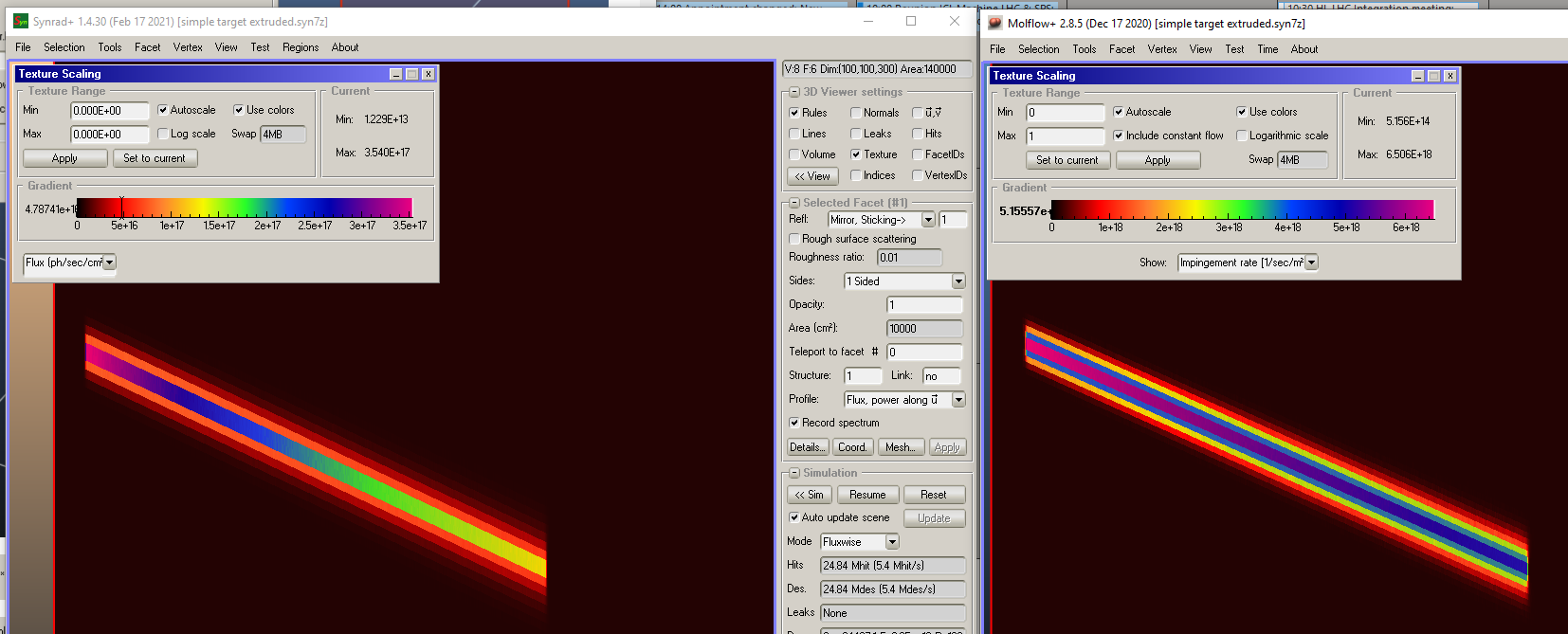
Flux is "compressed":

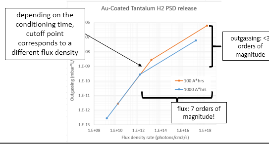
Synrad simulations: several orders of magnitude if possible: