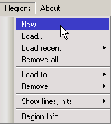
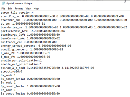
Synrad tutorial: Simple dipole with a target = In this example we'll create the first working Synrad simulation, equivalent to the "test pipe" in Molflow. By default, Synrad starts with an empty geometry, where we have to add regions, representing magnetic elements. We will add a single dipole: ## Adding a dipole In Synrad, each region has to be backed by a ```.param``` file on disk. 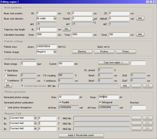Therefore, when choosing ```Regions/New```, you'll have to specify a location and a filename:  Once the location is defined, the region editor pops up to define the parameters:  Full info on the text fields is in the documentation [here](https://molflow.web.cern.ch/content/documentation-region-editor). The parameters that we'll set are: - **Beam start position**: in centimeters. We'll set X,Y,Z = 0,0,0 - **Beam start direction**: in the Z direction (corresponding to theta=alpha=0) - **Trajectory step length**: Synrad approximates all magnetic elements by short, straight sections, then recalculates the (curved) beam direction. We'll aim for around a 1000 points by choosing step length=0.1cm - **Calculation boundary**: currently magnetic regions are defined by their limit (not their length). The first of the X,Y,Z coordinates that will be hit will stop the calculation. We start the element at 0,0,0 and since it is 1m long, the boundary is (X=1000,Y=1000,Z=100), of which the Z boundary will be hit first. - **Particle mass and charge**: click ```Electron```. - **Beam energy**: in our simple system it will be 1GeV - **Beam current**: 100mA - **Lattice functions**: We'll use "Ideal beam" in this example, resulting in 0 beam width - **Photon generation**: We can restrict the SR spectrum to between two energies. 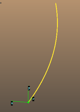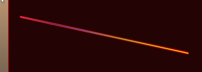(The SR spectrum is "infinite" in the lower energy direction and has a sharp cutoff in the high energy region) - **Magnetic field**: we'll put a constant magnetic field of 1T in the Y direction Clicking Apply&Recalculate we can see the curvature of the dipole:   Note that the GUI is just a front-end to the ```.param``` file, which can be viewed and edited directly in a text editor (save and reload if you do that and Synrad will take changes into account).  **Note about the location of the ```.param``` files**: They are saved to your specified location. However, if you save the whole geometry as a compressed ```.syn7z``` file, they are packaged with the file (a copy is made). After opening the syn7z file, the param files will be in a temporary directory.  After changing and saving the edited file, the Reload file button parses it again and calculates the points.  You have a tool to see the trajectory points (View points) in the region edtior.  Clicking on a row displays the point, clicking on a point with the *trajectory selector* tool in the 3D scene selects it in the point view dialog.  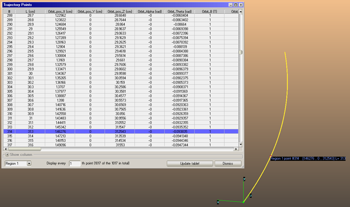The trajectory selector tool is next to the vertex selector tool.  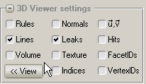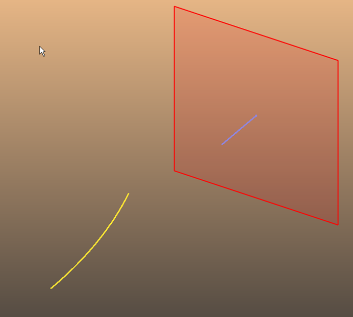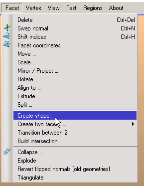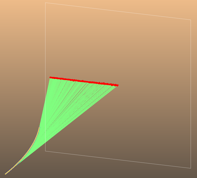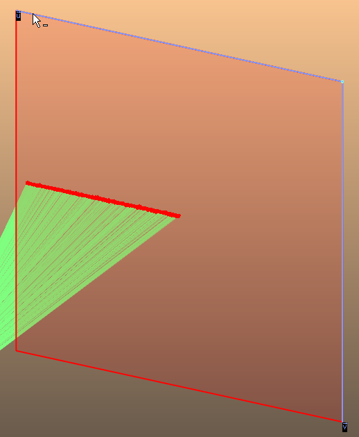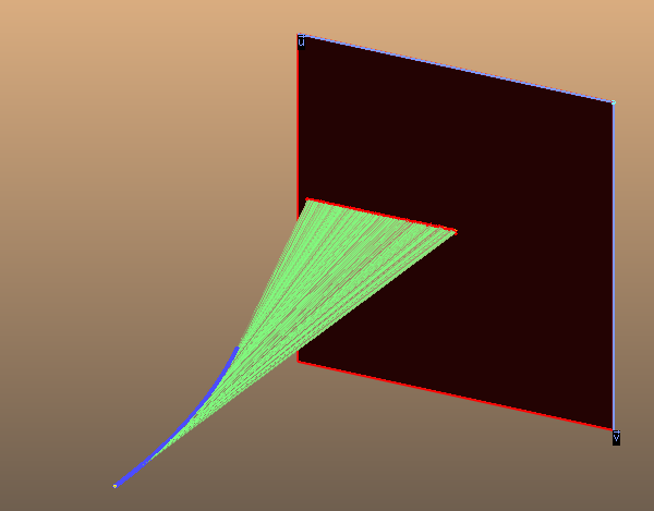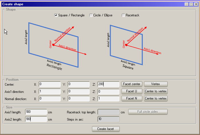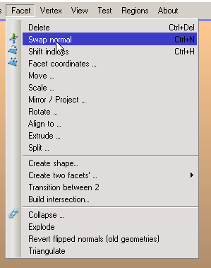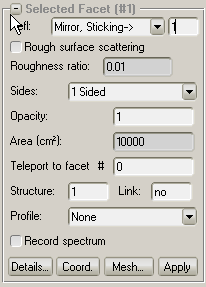## Starting the simulation Turn on leak display (no geometry yet):  You can see that the trajectory creates photons, which cause leaks for the moment:  ## Adding a target Use the Facet / Create shape tool:  Create a 100x100 cm square at Z=200cm  Make its normal point towards the dipole:   Add sticking to it so it absorbs photons:  Your simulation is now running:  ## Record spectrum Turn on the Record spectrum property for the facet:  Add the curve to the plotter:   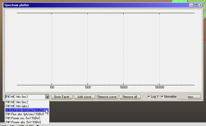The plotted spectrum:  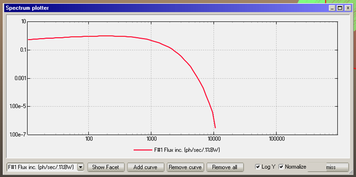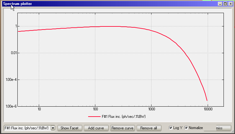We can see that photons are recorded until 1MeV whereas they are generated until ~10keV. 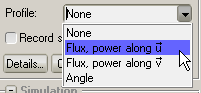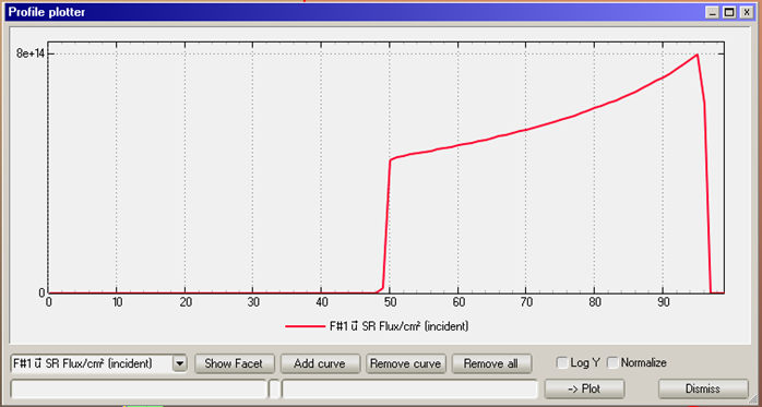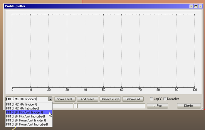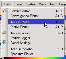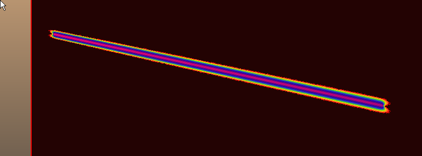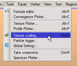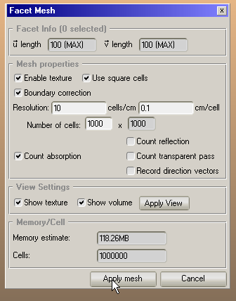Let's restrict the generation range:    Now the spectrum is filling the recorded range better:  ## Add a profile Turn on u,v view:  We'll plot the profile in the u direction:   Add the curve to the profile plotter:    ## Adding textures In Synrad there isn't (yet) an "<< Adv" button for the advanced facet parameters. Use the Mesh... 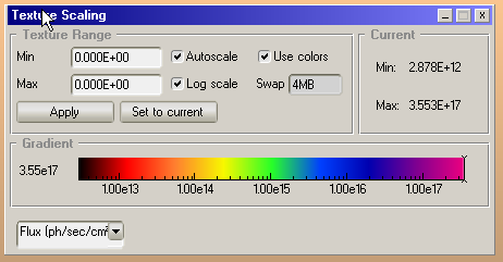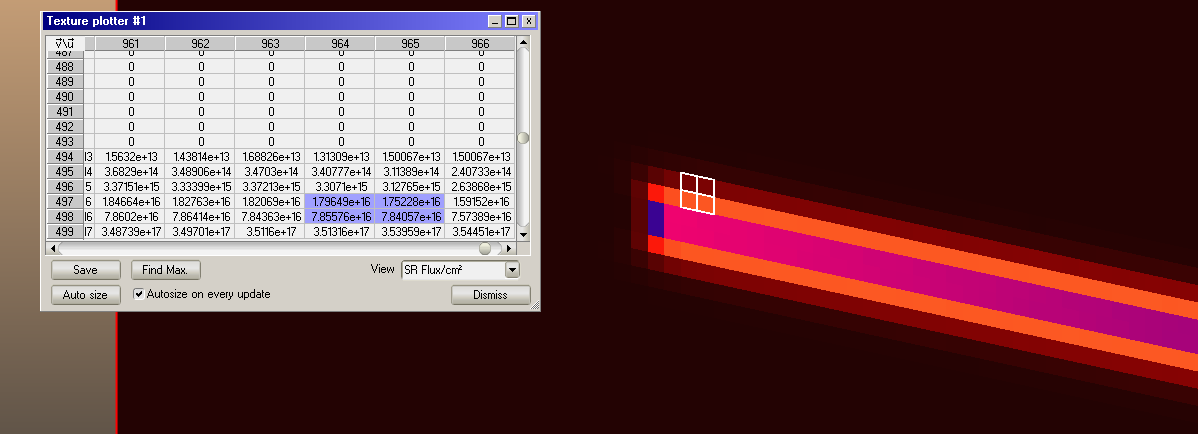button to add a texture:  Let's use 10 cells/cm:   Turn off lines view and zoom in on the texture:  Make the scale logarithmic:   linear scale:   Selecting a cell or block of cells in the Texture plotter displays it in the 3D scene: