# Advanced Accelerator Physics CAS 2019, Optics Design
During the [CAS 2019](https://cas.web.cern.ch/schools/slangerup-2019) in Slangerup, we will use Python as scripting language for the *Optics Design and Correction* afternoon course. The *Optics Design and Correction* is one out of the three parallel afternoon courses. If you choose to attend this course, we kindly ask you to make some homework before coming to Slangerup to prepare yourself (and your laptop) for the course.
For this course a **basic knowledge of Python is assumed**, therefore if you are not familiar with it you can find, in the following sections, few resources to fill the gap. During the course we will use Python3 in a Jupyter notebook and, mostly, the *numpy*, *matplotlib*, *pandas*, *sympy*, *PyNAFF* and *cpymad* packages. We will explain in the following sections how to install this software on your laptops.
After a short introduction where we provided some useful links to get familiar with Python, we will focus on the software setup. Depending on your operating systems (we will consider OSX, Windows and UNIX) you have different procedures to follow.
For **OSX** users, please follow the instructions in the *OSX: Install and run a Docker image* section.
For the **Windows** users, please follow the instructions in the *Windows: Docker Toolbox* section.
For **UNIX** users, please follow the instructions in the instructions in the *UNIX: Anaconda + cpymad* section.
# A (very) short introduction to Python
## Test Python on a web page
If you are not familiar with Python and you have not it installed on your laptop, you can start playing with simple python snippets on the web: without installing any special software you can connect, e.g., to
https://www.pythonanywhere.com/try-ipython/
and test the following commands
```python=
import numpy as np
# Matrix definition
Omega=np.array([[0, 1],[-1,0]])
M=np.array([[1, 0],[1,1]])
# Sum and multiplication of matrices
Omega - M.T @ Omega @ M
# M.T means the "traspose of M".
# Function definition
def Q(f=1):
return np.array([[1, 0],[-1/f,1]])
#Eigenvalues and eigenvectors
np.linalg.eig(M)
```
You can compare and check your output with the ones [here](https://cernbox.cern.ch/index.php/s/xipyXzX7V9KBJbI).
## The *numpy* package
To get familiar with the *numpy* package have a look at the following [summary poster](https://s3.amazonaws.com/assets.datacamp.com/blog_assets/Numpy_Python_Cheat_Sheet.pdf).
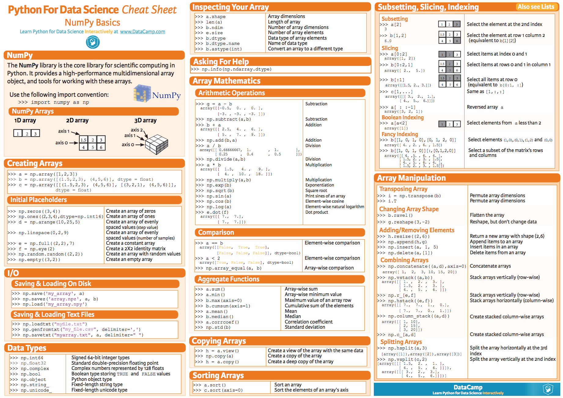
You can google many other resources, but the one presented of the poster cover the set of instructions you should familiar with.
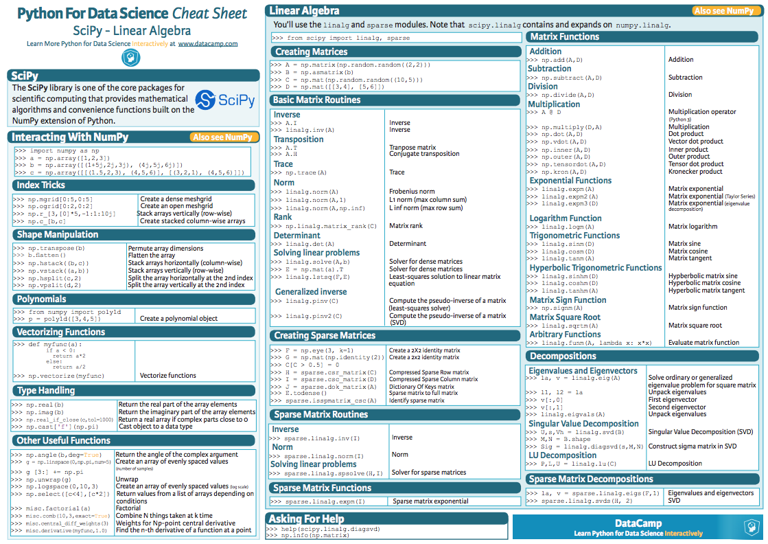
## The linalg module
To get familiar with the Linear Algebra (linalg) module have a look at the following [summary poster](
https://s3.amazonaws.com/assets.datacamp.com/blog_assets/Python_SciPy_Cheat_Sheet_Linear_Algebra.pdf).
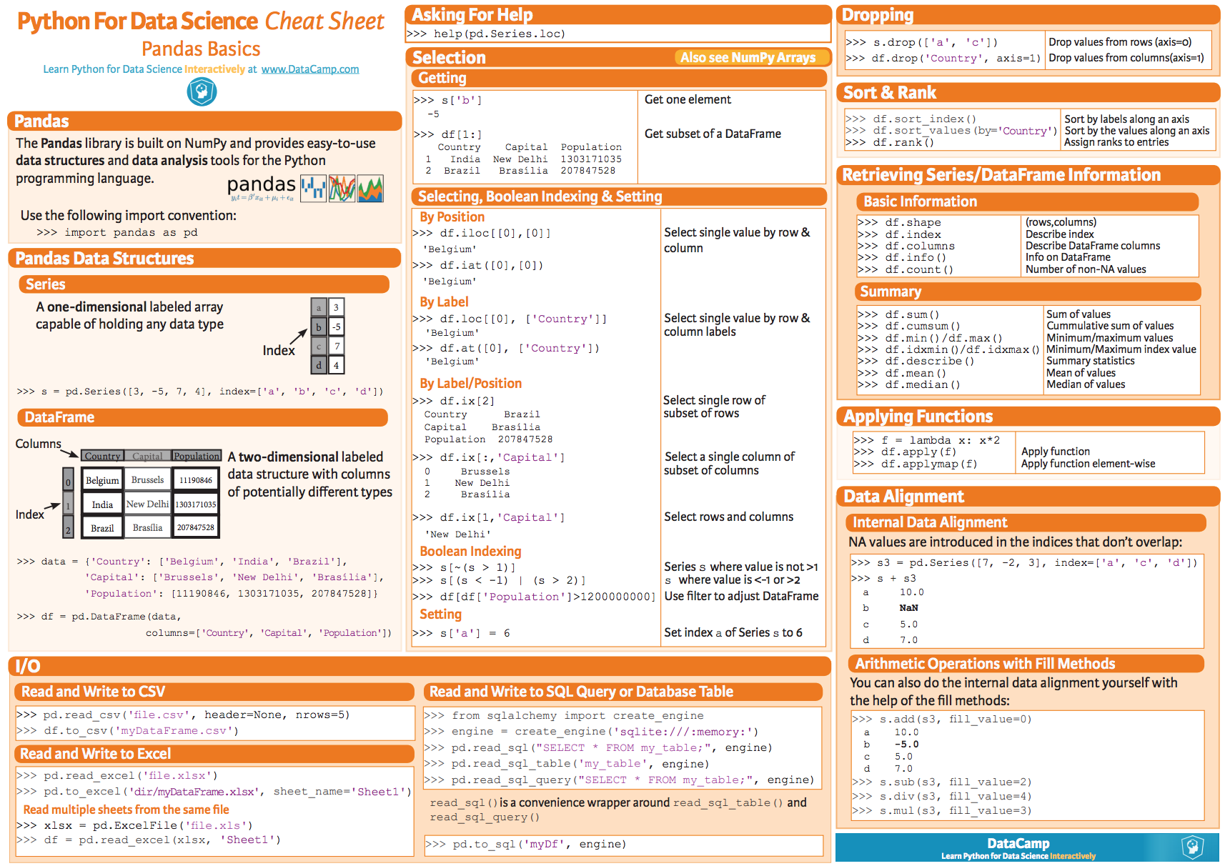
## The *pandas* package
To get familiar with the *pandas* package have a look at the following [summary poster](
https://s3.amazonaws.com/assets.datacamp.com/blog_assets/PandasPythonForDataScience.pdf).
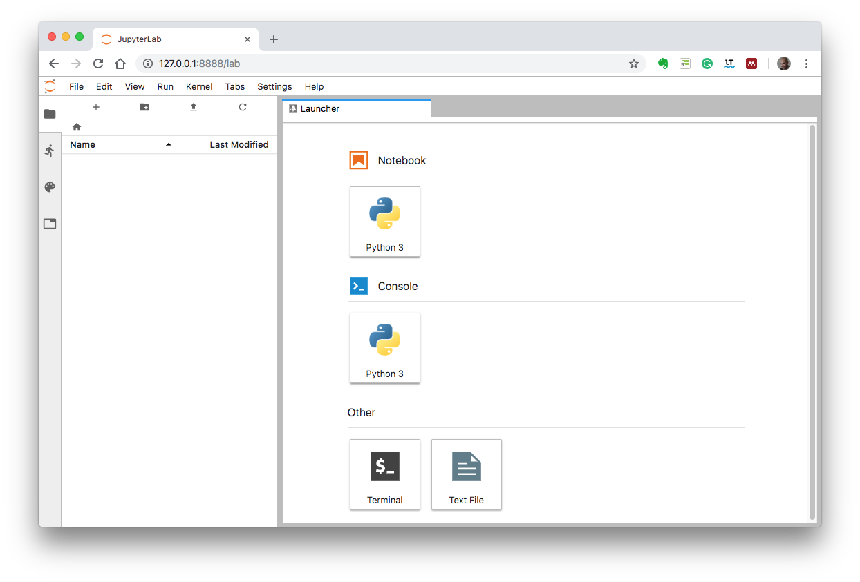
## JupyterLab
JupyterLab is a user-friendly environment to work with Python.
You can find an overview on JupyterLab [here](
https://jupyterlab.readthedocs.io/en/stable/).
In the following section we will explain how to install a Python on your laptop: we propose three different approaches for OSX, Windows and UNIX systems, respectively.
# OSX: install and run a Docker image
In order to ease the installation procedure, we prepared a virtual environment that launch a Python3 Jupyter server (the installation on *cpymad* on OSX can be tricky, so we suggest to use the Docker image).
### STEP 1: install the Docker Desktop
Please install the [Docker Desktop](https://www.docker.com/products/docker-desktop).
:::info
This is available for MAC and Windows 10 Enterprise and Professional (but not the 'Home Edition'). If you have Windows Home edition please refer to the *Windows: Docker Toolbox* section.
:::
### STEP 2: run the Docker image
Once the Docker Desktop is installed and running, open a terminal, move to a folder you want to use for CAS exercises and run the instruction
``` bash
>> docker run -p 8888:8888 -v "$PWD":/cas sterbini/cas_aap_2019
```
This will download the image (~5GB): an internet connection is needed **only for the first time**, afterwords you can work offline.
:::warning
It is very important to have an offline working solution. Our experience with the previous schools showed that the standard WiFi infrastructure does not always meet the needed bandwidth performance. So, even if you have a working online Python environment (e.g. https://swan.web.cern.ch/) we strongly encourage to use an offline Python distribution.
:::
You should get something as
```bash
MACBE16107:Tutorials sterbini$ docker run -p 8888:8888 -v "$PWD":/cas sterbini/cas_aap_2019
[I 08:37:31.108 LabApp] Writing notebook server cookie secret to /cas/.local/share/jupyter/runtime/notebook_cookie_secret
[I 08:37:31.341 LabApp] JupyterLab extension loaded from /opt/conda/lib/python3.6/site-packages/jupyterlab
[I 08:37:31.341 LabApp] JupyterLab application directory is /opt/conda/share/jupyter/lab
[W 08:37:31.343 LabApp] JupyterLab server extension not enabled, manually loading...
[I 08:37:31.353 LabApp] JupyterLab extension loaded from /opt/conda/lib/python3.6/site-packages/jupyterlab
[I 08:37:31.353 LabApp] JupyterLab application directory is /opt/conda/share/jupyter/lab
[I 08:37:31.354 LabApp] Serving notebooks from local directory: /cas
[I 08:37:31.354 LabApp] The Jupyter Notebook is running at:
[I 08:37:31.354 LabApp] http://(4bd247dca0ba or 127.0.0.1):8888/?token=ea65f062bfce037fd7a3b47926393a0d5ded381785b0136b
[I 08:37:31.355 LabApp] Use Control-C to stop this server and shut down all kernels (twice to skip confirmation).
[C 08:37:31.364 LabApp]
Copy/paste this URL into your browser when you connect for the first time,
to login with a token:
http://(4bd247dca0ba or 127.0.0.1):8888/?token=ea65f062bfce037fd7a3b47926393a0d5ded381785b0136b
```
:::info
**The last line is the most important one**.
:::
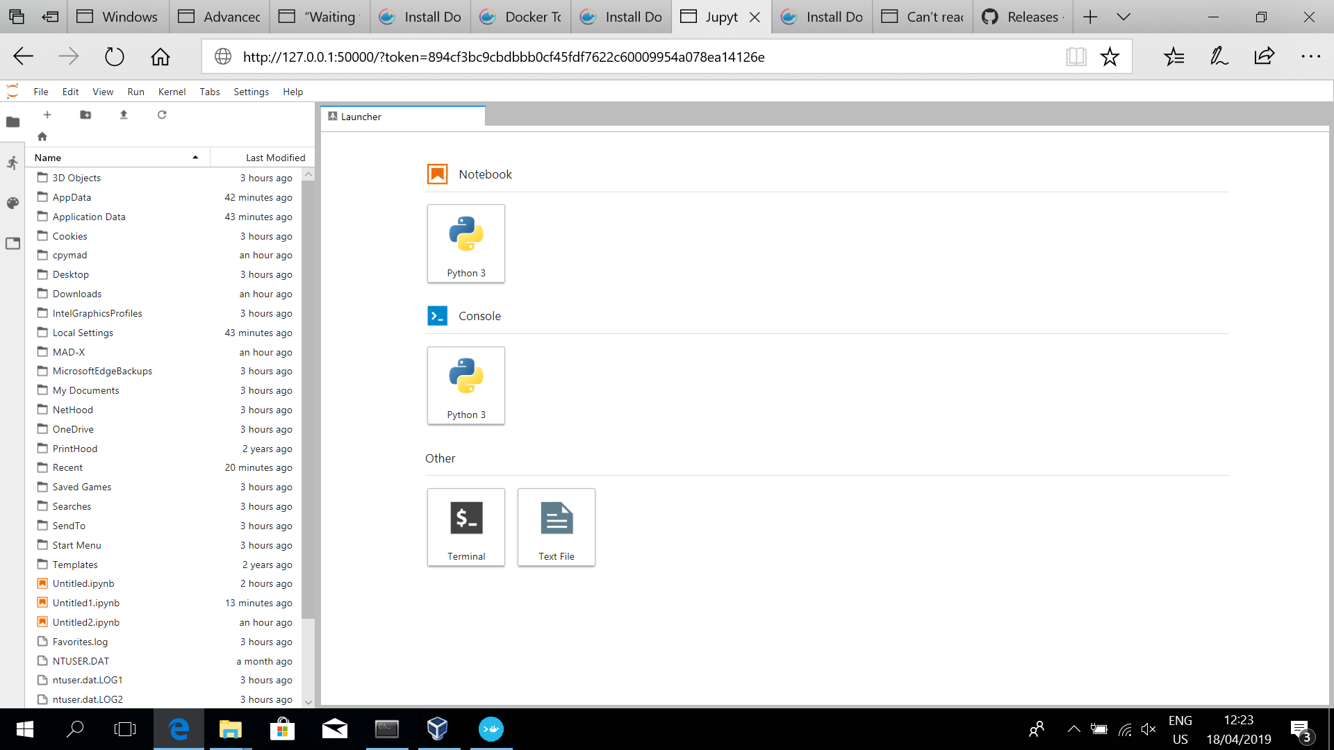
### STEP 3: open JupyterLab from a browser
Open a web browser and connect to the python server at (**in this case**, check the last line)
http://127.0.0.1:8888/?token=ea65f062bfce037fd7a3b47926393a0d5ded381785b0136b
You have to copy, paste and **edit** the last line on the address field of your browser.
You should see something as
This JupyterLab environment is setup with the software needed for the Optics course.
The *Laucher* tab allows you to open a notebook or console or some basic terminal/editing environment.
You can clic on the *Python 3 Notebook* icon in the *Launcher* tab and test the code example at the end of this document to verify that everything is working as expected.
# UNIX: Anaconda distribution
For UNIX system the simplest way to install Python environment on your laptop is to setup manually your environment by installing [*anaconda*](http://docs.continuum.io/_downloads/9ee215ff15fde24bf01791d719084950/Anaconda-Starter-Guide.pdf) from
http://docs.continuum.io/anaconda/
### STEP 1: Anaconda installation
We suggest to install the Python 3.7 version (2019.03)
https://www.anaconda.com/distribution/
List the packages that are installed with
```
>> conda list
```
and verify that you have *matplotlib*, *numpy*, *scipy*, *pandas*, *sympy*.
If some of them are missing, please install them with, e.g.,
```
>> conda install -c conda-forge matplotlib
```
### STEP 2: *PyNAFF* installation
You can find information on https://pypi.org/project/PyNAFF/.
In most of the case it is enough to open a terminal and do
```
>> pip install PyNAFF
```
### STEP 3: *cpymad* installation
The standard *anaconda* distribution comes with most of the needed packages but *cpymad*. You can install it following the instructions from https://github.com/hibtc/cpymad. In most of the case it is enough to open a terminal and do
```
>> pip install cpymad
```
### STEP 4: JupyterLab
Now you can launch from a terminal JupyterLab
```
>> jupyter-lab
```
:::info
If JupyterLab is not installed in your system you can install it with
```
>> conda install -c conda-forge jupyterlab
```
:::
The *jupyter-lab* command will open a browser.
The Laucher tab allows you to open a notebook or console or some basic terminal/editing environment.
You can clic on the Python 3 Notebook icon in the Launcher tab and test the code example at the end of this document to verify that everything is working as expected.
# Windows: Docker Toolbox
If you have Windows 10 Professional or Enterprise you can follow the instructions given for OSX. The other Windows versions are not compatible with **Docker Desktop**.
In alternative to **Docker Desktop**, there is a legacy software caller **Docker Toolbox** (we tested it on Windons 10 Home). This comes with an Oracle Virtual Box where you will run the Docker Image.
### STEP 1: Docker Toolbox installation
Download **Docker Toolbox** from https://github.com/docker/toolbox/releases/download/v18.09.3/DockerToolbox-18.09.3.exe
Install it (using custom configuration).
### STEP 2: redirect the port 8888
You have to redirect the port 8888 of the virtual machine to the localhost port 50000 (you can use another free port if you like or if port the 50000 is already in use). This can be done from the Oracle VM VirtualBox (icon on your desktop) accessing the menu of the default Virtual machine:
'Settings'->-'Network'->-'Advanced'->-'Port Forwarding'.
Add ('+' icon on the top/right) a rule as shown in the following screenshot
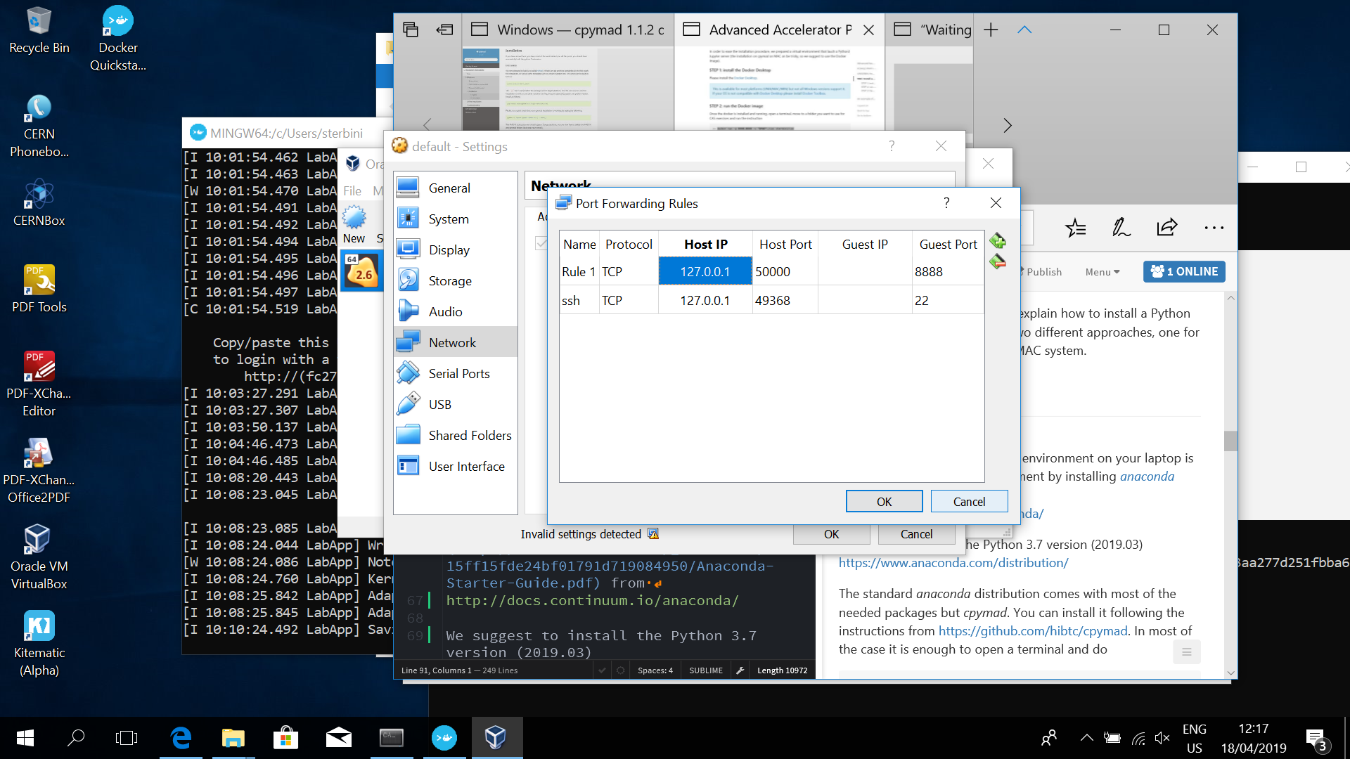
This means that you can access the port 8888 of the virtual machine from the port 50000 of the localhost (127.0.0.1).
### STEP 3: install and launch the docker image
Now open the Docker Quickstart (icon on the Desktop). It will take some time to start the virtual machine. Then move to your home folder typing
```bash
>> cd
```
Then type
```bash
>> docker run -p 8888:8888 -v "$PWD":/cas sterbini/cas_aap_2019
```
This download the docker image (only for the first time, ~5 GB) and run it.
You will get something like
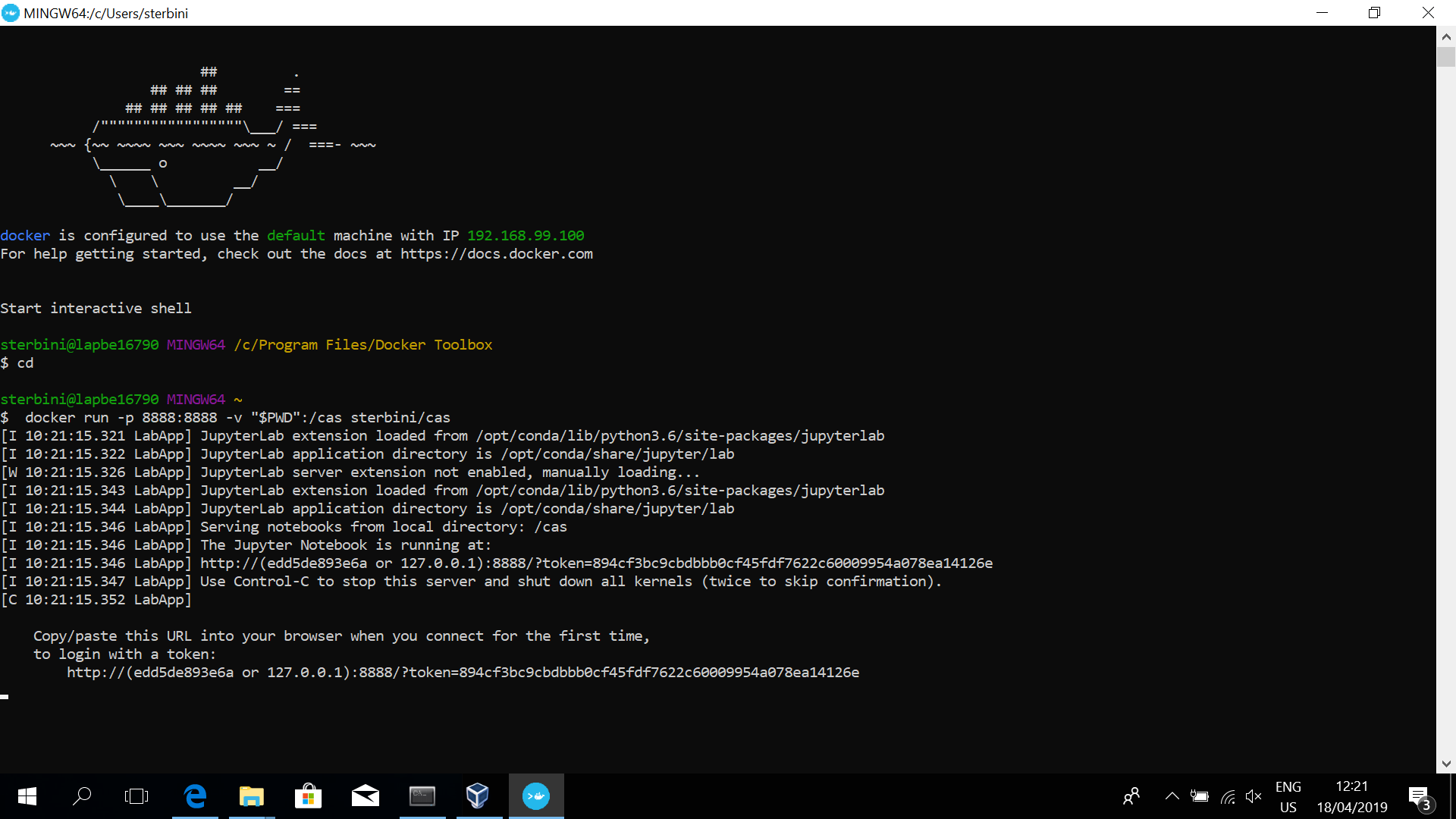
:::info
**The last line is the most important one**.
:::
### STEP 4: open JupyterLab from a browser
Open a web browser and connect to the python server at (**in this case**, see the last line of the previous screenshot)
http://127.0.0.1:50000/?token=HereGoesYourAlphanumericToken
:::danger
You have to copy, paste and **edit** the last line on the address field of your browser. **Please remember to replace the port 8888 with the port 50000.**
:::
It will open a browser and you should get something as
The Laucher tab allows you to open a notebook or console or some basic terminal/editing environment.
You can clic on the Python 3 Notebook icon in the Launcher tab and test the code example at the end of this document to verify that everything is working as expected.
# An example of Python3 notebook in Jupyter Lab.
From the *Launcher* of JupyterLab select the Python 3 Notebook.
You can import the python library of MAD-X (*cpymad*) with the following command.
```python
from cpymad.madx import Madx
from matplotlib import pyplot as plt
myMad = Madx()
```
and now you can twiss a simple FODO cell (more details during the course) with the following code
``` python
myString='''
! *********************************************************************
! Second part
! *********************************************************************
! *********************************************************************
! Definition of parameters
! *********************************************************************
l_cell=100;
quadrupoleLenght=5;
f=200;
myK:=1/f/quadrupoleLenght;// m^-2
! *********************************************************************
! Definition of magnet
! *********************************************************************
QF: quadrupole, L=quadrupoleLenght, K1:=myK;
QD: quadrupole, L=quadrupoleLenght, K1:=-myK;
! *********************************************************************
! Definition of sequence
! *********************************************************************
myCell:sequence, refer=entry, L=L_CELL;
quadrupole1: QF, at=0;
marker1: marker, at=25;
quadrupole2: QD, at=50;
endsequence;
! *********************************************************************
! Definition of beam
! *********************************************************************
beam, particle=proton, energy=2;
! *********************************************************************
! Use of the sequence
! *********************************************************************
use, sequence=myCell;
! *********************************************************************
! TWISS
! *********************************************************************
title, 'My first twiss';
twiss, file=myFirstTwiss.twiss;
'''
myMad.input(myString);
```
You can see the *Q1* and *betymax* parameters by executing this cell
``` python
myString='''
value, table(SUMM,Q1);
value, table(SUMM,betymax);
'''
myMad.input(myString);
```
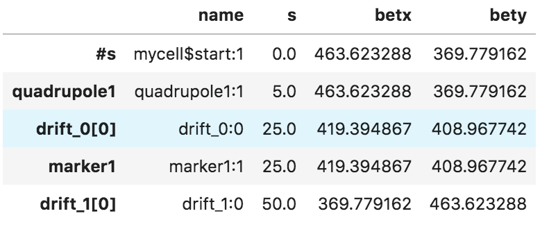
and you can get a pandas dataframe with the information of the lattice by
``` python
myDF=myMad.table.twiss.dframe()
myDF[['name','s','betx','bety']].head()
```
You should get something like
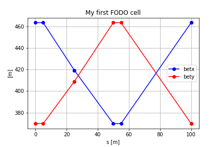
To plot some data of the *twiss* table you can execute
``` python
plt.plot(myDF['s'],myDF['betx'],'ob-')
plt.plot(myDF['s'],myDF['bety'],'or-')
plt.legend()
plt.grid()
plt.xlabel('s [m]')
plt.ylabel('[m]')
plt.title('My first FODO cell')
```
You can do also a bit of symbolic computation with
``` python
import sympy as sy
import numpy as np
from sympy import init_session
init_session()
la=np.linalg
L_cell=sy.Symbol('L_cell', positive=True);
f_1=sy.Symbol('f_1', positive=True);
f_2=sy.Symbol('f_2', positive=True);
f=sy.Symbol('f', positive=True);
QF=sy.Matrix([[1,0], [-1/f,1]])
DRIFT=sy.Matrix([[1,L_cell/2], [0,1]])
QD=sy.Matrix([[1,0], [1/f,1]])
# This is the OTM
M=DRIFT@QD@DRIFT@QF
M=sy.simplify(M)
M
```
or FTT analysis using PyNAFF, e.g.,
``` python
import PyNAFF as pnf
import numpy as np
t = np.linspace(1, 3000, num=3000, endpoint=True)
Q = 0.12345
signal = np.sin(2.0*np.pi*Q*t)
pnf.naff(signal, 500, 1, 0 , False, window=1)
# outputs an array of arrays for each frequency. Each sub-array includes:
# [order of harmonic, frequency, Amplitude, Re{Amplitude}, Im{Amplitude]
# My frequency is simply
pnf.naff(signal, 500, 1, 0 , False)[0][1]
```
An example of test ipython notebook is shown in
https://cernbox.cern.ch/index.php/s/JJCu7KRPAjuitVF
You will learn much more at Slangerup. **See you there!**